scipy.interpolate.

spalde

scipy.interpolate.spalde(x, tck)

Evaluate a B-spline and all its derivatives at one point (or set of points) up to order k (the degree of the spline), being 0 the spline itself.

Legacy

This function is considered legacy and will no longer receive updates. While we currently have no plans to remove it, we recommend that new code uses more modern alternatives instead. Specifically, we recommend constructing a BSpline object and evaluate its derivative in a loop or a list comprehension.

Parameters:

xarray_like

A point or a set of points at which to evaluate the derivatives. Note that t(k) <= x <= t(n-k+1) must hold for each x.

tcktuple

A tuple (t,c,k) containing the vector of knots, the B-spline coefficients, and the degree of the spline whose derivatives to compute.

Returns:

results{ndarray, list of ndarrays}

An array (or a list of arrays) containing all derivatives up to order k inclusive for each point x, being the first element the spline itself.

See also

splprep, splrep, splint, sproot, splev, bisplrep, bisplev

UnivariateSpline, BivariateSpline

References

[1]

de Boor C : On calculating with b-splines, J. Approximation Theory 6 (1972) 50-62.

[2]

Cox M.G. : The numerical evaluation of b-splines, J. Inst. Maths applics 10 (1972) 134-149.

[3]

Dierckx P. : Curve and surface fitting with splines, Monographs on Numerical Analysis, Oxford University Press, 1993.

Examples

Try it in your browser!

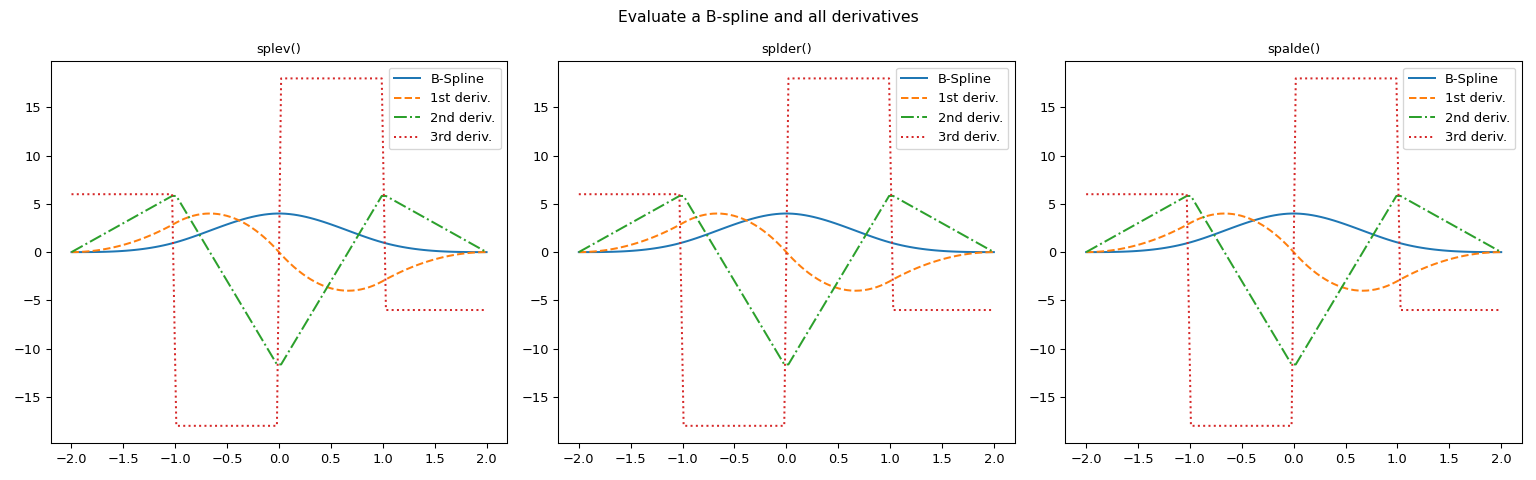
To calculate the derivatives of a B-spline there are several aproaches. In this example, we will demonstrate that spalde is equivalent to calling splev and splder.

>>> import numpy as np
>>> import matplotlib.pyplot as plt
>>> from scipy.interpolate import BSpline, spalde, splder, splev

>>> # Store characteristic parameters of a B-spline
>>> tck = ((-2, -2, -2, -2, -1, 0, 1, 2, 2, 2, 2),  # knots
...        (0, 0, 0, 6, 0, 0, 0),  # coefficients
...        3)  # degree (cubic)
>>> # Instance a B-spline object
>>> # `BSpline` objects are preferred, except for spalde()
>>> bspl = BSpline(tck[0], tck[1], tck[2])
>>> # Generate extra points to get a smooth curve
>>> x = np.linspace(min(tck[0]), max(tck[0]), 100)

Evaluate the curve and all derivatives

>>> # The order of derivative must be less or equal to k, the degree of the spline
>>> # Method 1: spalde()
>>> f1_y_bsplin = [spalde(i, tck)[0] for i in x ]  # The B-spline itself
>>> f1_y_deriv1 = [spalde(i, tck)[1] for i in x ]  # 1st derivative
>>> f1_y_deriv2 = [spalde(i, tck)[2] for i in x ]  # 2nd derivative
>>> f1_y_deriv3 = [spalde(i, tck)[3] for i in x ]  # 3rd derivative
>>> # You can reach the same result by using `splev`and `splder`
>>> f2_y_deriv3 = splev(x, bspl, der=3)
>>> f3_y_deriv3 = splder(bspl, n=3)(x)

>>> # Generate a figure with three axes for graphic comparison
>>> fig, (ax1, ax2, ax3) = plt.subplots(1, 3, figsize=(16, 5))
>>> suptitle = fig.suptitle(f'Evaluate a B-spline and all derivatives')
>>> # Plot B-spline and all derivatives using the three methods
>>> orders = range(4)
>>> linetypes = ['-', '--', '-.', ':']
>>> labels = ['B-Spline', '1st deriv.', '2nd deriv.', '3rd deriv.']
>>> functions = ['splev()', 'splder()', 'spalde()']
>>> for order, linetype, label in zip(orders, linetypes, labels):
...     ax1.plot(x, splev(x, bspl, der=order), linetype, label=label)
...     ax2.plot(x, splder(bspl, n=order)(x), linetype, label=label)
...     ax3.plot(x, [spalde(i, tck)[order] for i in x], linetype, label=label)
>>> for ax, function in zip((ax1, ax2, ax3), functions):
...     ax.set_title(function)
...     ax.legend()
>>> plt.tight_layout()
>>> plt.show()

Go BackOpen In Tab