scipy.interpolate.

lagrange#

scipy.interpolate.lagrange(x, w)[source]#

Return a Lagrange interpolating polynomial.

Given two 1-D arrays x and w, returns the Lagrange interpolating polynomial through the points (x, w).

Warning: This implementation is numerically unstable. Do not expect to be able to use more than about 20 points even if they are chosen optimally.

Deprecated since version 1.18.0: This function is deprecated and will be removed in SciPy 1.20.0. Use scipy.interpolate.BarycentricInterpolator instead.

Parameters:

xarray_like: x represents the x-coordinates of a set of datapoints.
warray_like: w represents the y-coordinates of a set of datapoints, i.e., f(x).

Returns:

lagrangenumpy.poly1d instance: The Lagrange interpolating polynomial.

Notes

The name of this function refers to the fact that the returned object represents a Lagrange polynomial, the unique polynomial of lowest degree that interpolates a given set of data [1]. It computes the polynomial using Newton’s divided differences formula [2]; that is, it works with Newton basis polynomials rather than Lagrange basis polynomials. For numerical calculations, the barycentric form of Lagrange interpolation (scipy.interpolate.BarycentricInterpolator) is typically more appropriate.

Array API Standard Support

lagrange is not in-scope for support of Python Array API Standard compatible backends other than NumPy.

See Support for the array API standard for more information.

References

[1]

Lagrange polynomial. Wikipedia. https://en.wikipedia.org/wiki/Lagrange_polynomial

[2]

Newton polynomial. Wikipedia. https://en.wikipedia.org/wiki/Newton_polynomial

Examples

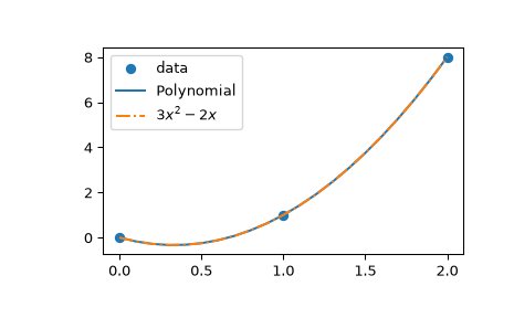
Interpolate \(f(x) = x^3\) by 3 points.

>>> import numpy as np
>>> from scipy.interpolate import lagrange
>>> x = np.array([0, 1, 2])
>>> y = x**3
>>> poly = lagrange(x, y)

Since there are only 3 points, the Lagrange polynomial has degree 2. Explicitly, it is given by

\[\begin{split}\begin{aligned} L(x) &= 1\times \frac{x (x - 2)}{-1} + 8\times \frac{x (x-1)}{2} \\ &= x (-2 + 3x) \end{aligned}\end{split}\]

>>> from numpy.polynomial.polynomial import Polynomial
>>> Polynomial(poly.coef[::-1]).coef
array([ 0., -2.,  3.])

>>> import matplotlib.pyplot as plt
>>> x_new = np.arange(0, 2.1, 0.1)
>>> plt.scatter(x, y, label='data')
>>> plt.plot(x_new, Polynomial(poly.coef[::-1])(x_new), label='Polynomial')
>>> plt.plot(x_new, 3*x_new**2 - 2*x_new + 0*x_new,
...          label=r"$3 x^2 - 2 x$", linestyle='-.')
>>> plt.legend()
>>> plt.show()

../../_images/scipy-interpolate-lagrange-1.png