scipy.interpolate.

BarycentricInterpolator#

class scipy.interpolate.BarycentricInterpolator(xi, yi=None, axis=0, *, wi=None, rng=None)[source]#

Barycentric (Lagrange with improved stability) interpolator (C∞ smooth).

Constructs a polynomial that passes through a given set of points. Allows evaluation of the polynomial and all its derivatives, efficient changing of the y-values to be interpolated, and updating by adding more x- and y-values. For numerical stability, a barycentric representation is used rather than computing the coefficients of the polynomial directly.

Parameters:

xiarray_like, shape (npoints, )

1-D array of x-coordinates of the points the polynomial should pass through

yiarray_like, shape (…, npoints, …), optional

N-D array of y-coordinates of the points the polynomial should pass through. If None, the y values will be supplied later via the set_y method. The length of yi along the interpolation axis must be equal to the length of xi. Use the axis parameter to select correct axis.

axisint, optional

Axis in the yi array corresponding to the x-coordinate values. Defaults to axis=0.

wiarray_like, optional

The barycentric weights for the chosen interpolation points xi. If absent or None, the weights will be computed from xi (default). This allows for the reuse of the weights wi if several interpolants are being calculated using the same nodes xi, without re-computation. This also allows for computing the weights explicitly for some choices of xi (see notes).

rng{None, int, numpy.random.Generator}, optional

If rng is passed by keyword, types other than numpy.random.Generator are passed to numpy.random.default_rng to instantiate a Generator. If rng is already a Generator instance, then the provided instance is used. Specify rng for repeatable interpolation.

If this argument random_state is passed by keyword, legacy behavior for the argument random_state applies:

If random_state is None (or numpy.random), the numpy.random.RandomState singleton is used.
If random_state is an int, a new RandomState instance is used, seeded with random_state.
If random_state is already a Generator or RandomState instance then that instance is used.

Changed in version 1.15.0: As part of the SPEC-007 transition from use of numpy.random.RandomState to numpy.random.Generator this keyword was changed from random_state to rng. For an interim period, both keywords will continue to work (only specify one of them). After the interim period using the random_state keyword will emit warnings. The behavior of the random_state and rng keywords is outlined above.

Attributes:

dtype

Methods

`__call__`(x)	Evaluate the interpolating polynomial at the points x
`add_xi`(xi[, yi])	Add more x values to the set to be interpolated
`derivative`(x[, der])	Evaluate a single derivative of the polynomial at the point x.
`derivatives`(x[, der])	Evaluate several derivatives of the polynomial at the point x
`set_yi`(yi[, axis])	Update the y values to be interpolated

Notes

This method is a variant of Lagrange polynomial interpolation [1] based on [2]. Instead of using Lagrange’s or Newton’s formula, the polynomial is represented by the barycentric formula

\[p(x) = \frac{\sum_{i=1}^m\ w_i y_i / (x - x_i)}{\sum_{i=1}^m w_i / (x - x_i)},\]

where \(w_i\) are the barycentric weights computed with the general formula

\[w_i = \left( \prod_{k \neq i} x_i - x_k \right)^{-1}.\]

This is the same barycentric form used by AAA and FloaterHormannInterpolator. However, in contrast, the weights \(w_i\) are defined such that \(p(x)\) is a polynomial rather than a rational function.

The barycentric representation avoids many of the problems associated with polynomial interpolation caused by floating-point arithmetic. However, it does not avoid issues that are intrinsic to polynomial interpolation. Namely, if the x-coordinates are equally spaced, then the weights can be computed explicitly using the formula from [2]

\[w_i = (-1)^i {n \choose i},\]

where \(n\) is the number of x-coordinates. As noted in [2], this means that for large \(n\) the weights vary by exponentially large factors, leading to the Runge phenomenon.

To avoid this ill-conditioning, the x-coordinates should be clustered at the endpoints of the interval. An excellent choice of points on the interval \([a,b]\) are Chebyshev points of the second kind

\[x_i = \frac{a + b}{2} + \frac{a - b}{2}\cos(i\pi/n).\]

in which case the weights can be computed explicitly as

\[\begin{split}w_i = \begin{cases} (-1)^i/2 & i = 0,n \\ (-1)^i & \text{otherwise} \end{cases}.\end{split}\]

See [2] for more infomation. Note that for large \(n\), computing the weights explicitly (see examples) will be faster than the generic formula.

References

[1]

https://en.wikipedia.org/wiki/Lagrange_polynomial

[2] (1,2,3,4)

Jean-Paul Berrut and Lloyd N. Trefethen, “Barycentric Lagrange Interpolation”, SIAM Review 2004 46:3, 501-517 DOI:10.1137/S0036144502417715

Examples

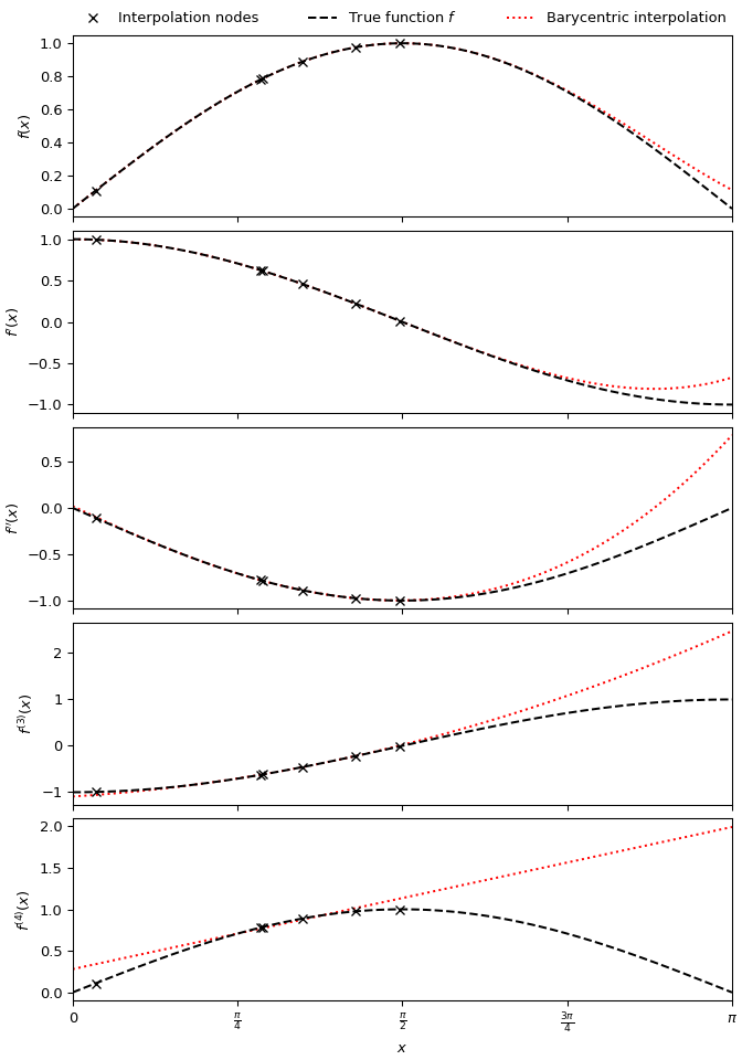
To produce a quintic barycentric interpolant approximating the function \(\sin x\), and its first four derivatives, using six randomly-spaced nodes in \((0, \pi/2)\):

>>> import numpy as np
>>> import matplotlib.pyplot as plt
>>> from scipy.interpolate import BarycentricInterpolator
>>> rng = np.random.default_rng()
>>> xi = rng.random(6) * np.pi/2
>>> f, f_d1, f_d2, f_d3, f_d4 = np.sin, np.cos, lambda x: -np.sin(x), lambda x: -np.cos(x), np.sin
>>> P = BarycentricInterpolator(xi, f(xi), random_state=rng)
>>> fig, axs = plt.subplots(5, 1, sharex=True, layout='constrained', figsize=(7,10))
>>> x = np.linspace(0, np.pi, 100)
>>> axs[0].plot(x, P(x), 'r:', x, f(x), 'k--', xi, f(xi), 'xk')
>>> axs[1].plot(x, P.derivative(x), 'r:', x, f_d1(x), 'k--', xi, f_d1(xi), 'xk')
>>> axs[2].plot(x, P.derivative(x, 2), 'r:', x, f_d2(x), 'k--', xi, f_d2(xi), 'xk')
>>> axs[3].plot(x, P.derivative(x, 3), 'r:', x, f_d3(x), 'k--', xi, f_d3(xi), 'xk')
>>> axs[4].plot(x, P.derivative(x, 4), 'r:', x, f_d4(x), 'k--', xi, f_d4(xi), 'xk')
>>> axs[0].set_xlim(0, np.pi)
>>> axs[4].set_xlabel(r"$x$")
>>> axs[4].set_xticks([i * np.pi / 4 for i in range(5)],
...                   ["0", r"$\frac{\pi}{4}$", r"$\frac{\pi}{2}$", r"$\frac{3\pi}{4}$", r"$\pi$"])
>>> for ax, label in zip(axs, ("$f(x)$", "$f'(x)$", "$f''(x)$", "$f^{(3)}(x)$", "$f^{(4)}(x)$")):
...     ax.set_ylabel(label)
>>> labels = ['Interpolation nodes', 'True function $f$', 'Barycentric interpolation']
>>> axs[0].legend(axs[0].get_lines()[::-1], labels, bbox_to_anchor=(0., 1.02, 1., .102),
...               loc='lower left', ncols=3, mode="expand", borderaxespad=0., frameon=False)
>>> plt.show()

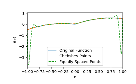
../../_images/scipy-interpolate-BarycentricInterpolator-1_00_00.png

Next, we show how using Chebyshev points of the second kind avoids the avoids the Runge phenomenon. In this example, we also compute the weights explicitly.

>>> n = 20
>>> def f(x): return np.abs(x) + 0.5*x - x**2
>>> i = np.arange(n)
>>> x_cheb = np.cos(i*np.pi/(n - 1))  # Chebyshev points on [-1, 1]
>>> w_i_cheb = (-1.)**i  # Explicit formula for weights of Chebyshev points
>>> w_i_cheb[[0, -1]] /= 2
>>> p_cheb = BarycentricInterpolator(x_cheb, f(x_cheb), wi=w_i_cheb)
>>> x_equi = np.linspace(-1, 1, n)
>>> p_equi = BarycentricInterpolator(x_equi, f(x_equi))
>>> xx = np.linspace(-1, 1, 1000)
>>> fig, ax = plt.subplots()
>>> ax.plot(xx, f(xx), label="Original Function")
>>> ax.plot(xx, p_cheb(xx), "--", label="Chebshev Points")
>>> ax.plot(xx, p_equi(xx), "--", label="Equally Spaced Points")
>>> ax.set(xlabel="$x$", ylabel="$f(x)$", xlim=[-1, 1])
>>> ax.legend()
>>> plt.show()

../../_images/scipy-interpolate-BarycentricInterpolator-1_01_00.png