ifht#
- scipy.fft.ifht(A, dln, mu, offset=0.0, bias=0.0)[source]#
Compute the inverse fast Hankel transform.
Computes the discrete inverse Hankel transform of a logarithmically spaced periodic sequence. This is the inverse operation to
fht.- Parameters:
- Aarray_like (…, n)
Real periodic input array, uniformly logarithmically spaced. For multidimensional input, the transform is performed over the last axis.
- dlnfloat
Uniform logarithmic spacing of the input array.
- mufloat
Order of the Hankel transform, any positive or negative real number.
- offsetfloat, optional
Offset of the uniform logarithmic spacing of the output array.
- biasfloat, optional
Exponent of power law bias, any positive or negative real number.
- Returns:
- aarray_like (…, n)
The transformed output array, which is real, periodic, uniformly logarithmically spaced, and of the same shape as the input array.
Notes
This function computes a discrete version of the Hankel transform
\[a(r) = \int_{0}^{\infty} \! A(k) \, J_\mu(kr) \, r \, dk \;,\]where \(J_\mu\) is the Bessel function of order \(\mu\). The index \(\mu\) may be any real number, positive or negative. Note that the numerical inverse Hankel transform uses an integrand of \(r \, dk\), while the mathematical inverse Hankel transform is commonly defined using \(k \, dk\).
See
fhtfor further details.Array API Standard Support
ifhthas experimental support for Python Array API Standard compatible backends in addition to NumPy. Please consider testing these features by setting an environment variableSCIPY_ARRAY_API=1and providing CuPy, PyTorch, JAX, or Dask arrays as array arguments. The following combinations of backend and device (or other capability) are supported.Library
CPU
GPU
NumPy
✅
n/a
CuPy
n/a
✅
PyTorch
✅
✅
JAX
✅
✅
Dask
⚠️ computes graph
n/a
See Support for the array API standard for more information.
Examples
>>> import numpy as np
>>> import matplotlib.pyplot as plt
>>> from scipy import fft
>>> from scipy.special import jv
Generate sample data
Aand evaluation pointskfor the Hankel transform of a signal.>>> k = np.logspace(-1, 1, 300) >>> A = np.zeros_like(k) >>> A[240] = 20
Calculate the logarithmic spacing of the elements in
Aand perform a second-order inverse Hankel transform on the sample data.>>> dln = np.log(k[1]/k[0]) >>> a = fft.ifht(A, dln, mu=2)
Calculate the evaluation points for the transformed data
a.ifhtcalculates evaluation pointsrsuch thatk * ris constant for eachkand then returns the transformed data in ascending order of evaluation points. To calculate the evaluation points in ascending order, flip the order ofkin the equation forr.>>> r = 1/np.flip(k)
Compare
awith the kernel function corresponding tok[240].>>> a_f = jv(2, k[240]*r)*r >>> fig, ax = plt.subplots() >>> ax.plot(r, a, label="ifht") >>> ax.plot(r, a_f, "--", label=r"$r J_2(k_{240} r)$") >>> ax.set_xlabel(r"$r$") >>> ax.set_ylabel("amplitude") >>> ax.legend() >>> plt.show()
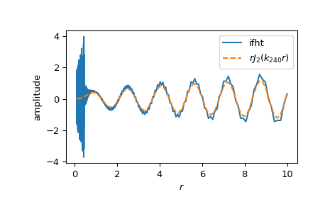
The plot shows that, for larger values of
r, the inverse Hankel transform follows the kernel function closely.