Skewness test#
This function tests the null hypothesis that the skewness of the population that the sample was drawn from is the same as that of a corresponding normal distribution.
Suppose we wish to infer from measurements whether the weights of adult human
males in a medical study are not normally distributed [1]. The weights (lbs)
are recorded in the array x below.
import numpy as np
x = np.array([148, 154, 158, 160, 161, 162, 166, 170, 182, 195, 236])
The skewness test scipy.stats.skewtest from [2] begins by computing a
statistic based on the sample skewness.
from scipy import stats
res = stats.skewtest(x)
res.statistic
np.float64(2.778857976990341)
Because normal distributions have zero skewness, the magnitude of this statistic tends to be low for samples drawn from a normal distribution.
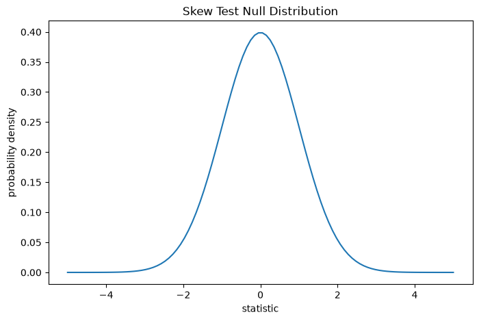
The test is performed by comparing the observed value of the statistic against the null distribution: the distribution of statistic values derived under the null hypothesis that the weights were drawn from a normal distribution.
For this test, the null distribution of the statistic for very large samples is the standard normal distribution.
import matplotlib.pyplot as plt
dist = stats.norm()
st_val = np.linspace(-5, 5, 100)
pdf = dist.pdf(st_val)
fig, ax = plt.subplots(figsize=(8, 5))

def st_plot(ax):  # we'll reuse this
    ax.plot(st_val, pdf)
    ax.set_title("Skew Test Null Distribution")
    ax.set_xlabel("statistic")
    ax.set_ylabel("probability density")

st_plot(ax)
plt.show()
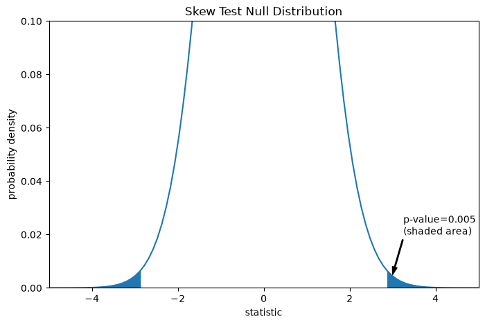
The comparison is quantified by the p-value: the proportion of values in the null distribution as extreme or more extreme than the observed value of the statistic. In a two-sided test, elements of the null distribution greater than the observed statistic and elements of the null distribution less than the negative of the observed statistic are both considered “more extreme”.
fig, ax = plt.subplots(figsize=(8, 5))
st_plot(ax)
pvalue = dist.cdf(-res.statistic) + dist.sf(res.statistic)
annotation = (f'p-value={pvalue:.3f}\n(shaded area)')
props = dict(facecolor='black', width=1, headwidth=5, headlength=8)
_ = ax.annotate(annotation, (3, 0.005), (3.25, 0.02), arrowprops=props)
i = st_val >= res.statistic
ax.fill_between(st_val[i], y1=0, y2=pdf[i], color='C0')
i = st_val <= -res.statistic
ax.fill_between(st_val[i], y1=0, y2=pdf[i], color='C0')
ax.set_xlim(-5, 5)
ax.set_ylim(0, 0.1)
plt.show()
res.pvalue
np.float64(0.00545503697474019)
If the p-value is “small” - that is, if there is a low probability of sampling data from a normally distributed population that produces such an extreme value of the statistic - this may be taken as evidence against the null hypothesis in favor of the alternative: the weights were not drawn from a normal distribution. Note that:
The inverse is not true; that is, the test is not used to provide evidence for the null hypothesis.
The threshold for values that will be considered “small” is a choice that should be made before the data is analyzed [3] with consideration of the risks of both false positives (incorrectly rejecting the null hypothesis) and false negatives (failure to reject a false null hypothesis).
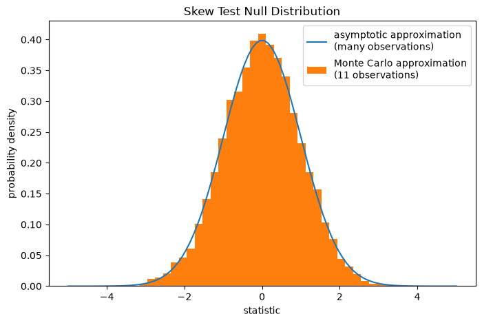
Note that the standard normal distribution provides an asymptotic approximation
of the null distribution; it is only accurate for samples with many
observations. For small samples like ours, scipy.stats.monte_carlo_test
may provide a more accurate, albeit stochastic, approximation of the exact
p-value.
def statistic(x, axis):
    # get just the skewtest statistic; ignore the p-value
    return stats.skewtest(x, axis=axis).statistic

res = stats.monte_carlo_test(x, stats.norm.rvs, statistic)
fig, ax = plt.subplots(figsize=(8, 5))
st_plot(ax)
ax.hist(res.null_distribution, np.linspace(-5, 5, 50),
        density=True)
ax.legend(['asymptotic approximation\n(many observations)',
           'Monte Carlo approximation\n(11 observations)'])
plt.show()
res.pvalue
np.float64(0.004)
In this case, the asymptotic approximation and Monte Carlo approximation agree fairly closely, even for our small sample.