Smoothing splines

Spline smoothing in 1D

For the interpolation problem, the task is to construct a curve which passes through a given set of data points. This may be not appropriate if the data is noisy: we may instead want to construct a smooth curve, \(g(x)\), which approximates the input data without passing through each point exactly.

To this end, scipy.interpolate allows constructing smoothing splines that balance how close the resulting curve, \(g(x)\), is to the data, and the smoothness of \(g(x)\). Mathematically, the task is to solve a penalized least-squares problem, where the penalty controls the smoothness of \(g(x)\).

We provide two approaches to constructing smoothing splines, which differ in (1) the form of the penalty term, and (2) the basis in which the smoothing curve is constructed. Below we consider these two approaches.

The former variant is performed by the make_smoothing_spline function, which is a clean-room reimplementation of the classic gcvspl Fortran package by H. Woltring. The latter variant is implemented by the make_splrep function, which is a reimplementation of the Fortran FITPACK library by P. Dierckx. A legacy interface to the FITPACK library is also available.

“Classic” smoothing splines and generalized cross-validation (GCV) criterion

Given the data arrays x and y and the array of non-negative weights, w, we look for a cubic spline function g(x) which minimizes

\[\sum\limits_{j=1}^n w_j \left\lvert y_j - g(x_j) \right\rvert^2 + \lambda\int\limits_{x_1}^{x_n} \left( g^{(2)}(u) \right)^2 d u\]

where \(\lambda \geqslant 0\) is a non-negative penalty parameter, and \(g^{(2)}(x)\) is the second derivative of \(g(x)\). The summation in the first term runs over the data points, \((x_j, y_j)\), and the integral in the second term is over the whole interval \(x \in [x_1, x_n]\).

Here the first term penalizes the deviation of the spline function from the data, and the second term penalizes large values of the second derivative—which is taken as the criterion for the smoothness of a curve.

There is a classic theorem (see, for example, Chapter 2 of [GS]) which says that the minimizer of this objective over all curves with a square-integrable second derivative is a natural cubic spline with knots at the data points, \(x_j\). The minimization space is not restricted to splines. It includes exponentials and any other curve the objective is defined for, and the minimizer still turns out to be a spline. The target function, \(g(x)\), is therefore taken to be exactly that, and the minimization is carried over the spline coefficients at a given value of \(\lambda\). (It is also possible to choose the knots differently, see the section on user provided knots below.)

Clearly, \(\lambda = 0\) corresponds to the interpolation problem—the result is a natural interpolating spline; in the opposite limit, \(\lambda \gg 1\), the result \(g(x)\) approaches a straight line (since the minimization effectively zeros out the second derivative of \(g(x)\)).

The smoothing function strongly depends on \(\lambda\), and multiple strategies are possible for selecting an “optimal” value of the penalty. One popular strategy is the so-called generalized cross-validation (GCV): conceptually, this is equivalent to comparing the spline functions constructed on reduced sets of data where we leave out one data point. Direct application of this leave-one-out cross-validation procedure is very costly, and we use a more efficient GCV algorithm.

To construct the smoothing spline given data and the penalty parameter, we use the function make_smoothing_spline. Its interface is similar to the constructor of interpolating splines, make_interp_spline: it accepts data arrays and returns a callable BSpline instance.

Additionally, it accepts an optional lam keyword argument to specify the penalty parameter \(\lambda\). If omitted or set to None, \(\lambda\) is computed via the GCV procedure.

To illustrate the effect of the penalty parameter, consider a toy example of a sine curve with some noise:

>>> import numpy as np
>>> from scipy.interpolate import make_smoothing_spline

Generate some noisy data:

>>> x = np.arange(0, 2*np.pi+np.pi/4, 2*np.pi/16)
>>> rng = np.random.default_rng()
>>> y =  np.sin(x) + 0.4*rng.standard_normal(size=len(x))

Construct and plot smoothing splines for a series of values of the penalty parameter:

>>> import matplotlib.pyplot as plt
>>> xnew = np.arange(0, 9/4, 1/50) * np.pi
>>> for lam in [0, 0.02, 10, None]:
...     spl = make_smoothing_spline(x, y, lam=lam)
...     plt.plot(xnew, spl(xnew), '-.', label=fr'$\lambda=${lam}')
>>> plt.plot(x, y, 'o')
>>> plt.legend()
>>> plt.show()

We clearly see that lam=0 constructs the interpolating spline; large values of lam flatten out the resulting curve towards a straight line; and the GCV result, lam=None, is close to the underlying sine curve.

User provided knot vectors

So far we never passed a knot vector to make_smoothing_spline, and rightly so. As discussed above, the minimizer of the smoothing objective has its knots at the data sites, so internally the knot vector was built to include all of x.

The fundamental issue with this is that the size of the system of equations is now in the hands of the size of the data. Every data site adds one basis function and one unknown to solve for. For large datasets it makes sense to sacrifice a little accuracy of the fitted curve for a smaller problem. For this reason make_smoothing_spline also accepts a user defined knot vector t. If the knots are chosen smartly, in most cases the harm is minimal.

A valid knot vector has its boundary knots repeated four times (more on this below), so throughout this section we use a small helper which adds the boundary knots to a vector of interior knots:

>>> import numpy as np
>>> from scipy.interpolate import make_smoothing_spline
>>> import matplotlib.pyplot as plt
>>>
>>> def clamped_knots(interior):
...     return np.concatenate([[x[0]] * 4, interior, [x[-1]] * 4])

Here is a minimal example:

>>> rng = np.random.default_rng(12345)
>>> x = np.linspace(0, 10, 50)
>>> y = np.sin(x) + 0.4 * rng.normal(size=len(x))
>>> # every other, third and fourth interior data site as knots
>>> t1 = clamped_knots(x[1:-1:2])
>>> t2 = clamped_knots(x[1:-1:3])
>>> t3 = clamped_knots(x[1:-1:4])
>>>
>>> xnew = np.linspace(x[0], x[-1], 400)
>>> for i, t in enumerate([t1, t2, t3]):
...     spl = make_smoothing_spline(x, y, lam=1e-3, t=t)
...     plt.plot(xnew, spl(xnew), label=f'$t_{i+1}$')
>>> plt.plot(x, y, 'o', alpha=0.4)
>>> plt.legend()
>>> plt.tight_layout()
>>> plt.show()

As seen in the plot above, the curves are pretty close to each other, even with roughly a quarter of the number of knots.

How do you select knots when the data is not equally distributed? Usually it is best to have more knots in the regions where the data is dense and fewer knots in the other places. A simple recipe is to place the knots at quantiles of x:

>>> rng = np.random.default_rng(12345)
>>> # data sites concentrated near the left end
>>> x = np.sort(10 * rng.random(100)**2)
>>> y = np.sin(x) + 0.4 * rng.normal(size=len(x))
>>>
>>> # 8 interior knots, placed two ways
>>> qs = np.linspace(0, 1, 10)[1:-1]
>>> t_eq = clamped_knots(np.linspace(x[0], x[-1], 10)[1:-1])
>>> t_qt = clamped_knots(np.quantile(x, qs, method='nearest'))
>>>
>>> xnew = np.linspace(x[0], x[-1], 400)
>>> for t, label in [(t_eq, 'equispaced knots'), (t_qt, 'knots at quantiles')]:
...     spl = make_smoothing_spline(x, y, lam=1e-3, t=t)
...     plt.plot(xnew, spl(xnew), label=label)
>>> plt.plot(x, y, 'o', alpha=0.4)
>>> plt.legend()
>>> plt.tight_layout()
>>> plt.show()

Both knot vectors have the same size and differ only in placement. The quantile based knots follow the density of the data, which is why that curve traces the local structure on the dense left side better. Note the method='nearest' argument, with it, numpy.quantile returns actual elements of x, so the knots are members of the data sites. Having knots at data sites is a convenience, not a requirement, the knots may be placed away from the data sites just as well.

Quantiles follow the density of the data. Another option is to follow the signal itself, more knots where the signal has features, fewer where it is quiet. Here the signal is flat except for a sharp bump, and we fit it twice with 8 interior knots, uniform versus placed around the bump:

>>> rng = np.random.default_rng(42)
>>> x = np.sort(rng.uniform(0, 1, 400))
>>> y = (0.3 + 0.25 * x + 0.45 * np.exp(-((x - 0.7) / 0.045)**2)
...      + rng.normal(0, 0.05, x.size))
>>>
>>> t_uniform = clamped_knots(np.linspace(x[0], x[-1], 10)[1:-1])
>>> t_placed = clamped_knots([0.25, 0.5, 0.62, 0.66, 0.70, 0.74, 0.78, 0.9])
>>>
>>> xnew = np.linspace(x[0], x[-1], 400)
>>> fig, axes = plt.subplots(1, 2, figsize=(10, 4), sharey=True)
>>> for ax, t, title in [(axes[0], t_uniform, 'uniform knots'),
...                      (axes[1], t_placed, 'placed knots')]:
...     spl = make_smoothing_spline(x, y, lam=1e-9, t=t)
...     ax.plot(x, y, 'o', alpha=0.3, markersize=3)
...     ax.plot(xnew, spl(xnew))
...     ax.plot(t[4:-4], np.full(len(t) - 8, 0.15), '|', markersize=10)
...     ax.set_title(title)
>>> plt.tight_layout()
>>> plt.show()

The uniform knots oversmooth the bump and wiggle in the quiet region. The placed knots are clustered around the bump, so the bump comes out clean and the rest stays calm.

The knots do not need to be a subset of the data sites, or coincide with them at all. Any non-decreasing knot vector works, as long as the boundary knots have multiplicity four (four because the splines here are cubic, in general it is k + 1) and all data sites lie within the base interval, t[3] <= x <= t[-4]. For instance, we can place the interior knots on a uniform grid that shares no points with x:

>>> t = clamped_knots(np.linspace(x[0], x[-1], 12)[1:-1])
>>> spl = make_smoothing_spline(x, y, lam=1e-3, t=t)

Finally, the default t=None corresponds to a specific choice of the knot vector, knots at all data sites, with the boundary ones repeated four times. Passing that vector explicitly reproduces the default result:

>>> t = clamped_knots(x[1:-1])
>>> spl_default = make_smoothing_spline(x, y, lam=1e-3)
>>> spl_user = make_smoothing_spline(x, y, lam=1e-3, t=t)
>>> xnew = np.linspace(x[0], x[-1], 400)
>>> np.allclose(spl_default(xnew), spl_user(xnew), atol=1e-12)
True

In other words, providing t generalizes the classic smoothing spline, you keep the same penalized least-squares problem, and additionally choose where the spline is allowed to bend.

Repeated interior knots

An interior knot may be repeated twice. Each repetition removes one continuity requirement, so a double knot allows the second derivative of the spline to jump at that point, while the spline and its slope stay continuous. This is useful when the underlying signal is known to change curvature abruptly somewhere, a single doubled knot at the breakpoint captures the feature, without spending extra knots everywhere else.

>>> rng = np.random.default_rng(12345)
>>> x = np.linspace(0, 10, 100)
>>> # flat for x < 5, parabolic for x > 5: the curvature jumps at 5
>>> signal = np.where(x < 5, 0.0, (x - 5)**2 / 5)
>>> y = signal + 0.15 * rng.normal(size=len(x))
>>>
>>> t_single = clamped_knots(np.linspace(1, 9, 5))
>>> # same knots, plus a second knot at the breakpoint x = 5
>>> t_double = np.sort(np.concatenate([t_single, [5.0]]))
>>>
>>> xnew = np.linspace(x[0], x[-1], 400)
>>> fig, (ax1, ax2) = plt.subplots(1, 2, figsize=(10, 4))
>>> for t, label in [(t_single, 'single knot at 5'),
...                  (t_double, 'double knot at 5')]:
...     spl = make_smoothing_spline(x, y, lam=1e-3, t=t)
...     ax1.plot(xnew, spl(xnew), label=label)
...     ax2.plot(xnew, spl.derivative(2)(xnew), label=label)
>>> ax1.plot(x, y, 'o', alpha=0.4)
>>> ax1.set_title('the fits (nearly identical)')
>>> ax2.axvline(5, color='k', ls=':', lw=1)
>>> ax2.set_title('second derivative')
>>> ax1.legend()
>>> plt.tight_layout()
>>> plt.show()

Notice that the two fits look nearly the same, the real difference shows up in the second derivative plot. With a single knot the second derivative has to change continuously, so the curvature change gets spread over the neighboring intervals. With the double knot it simply jumps at the breakpoint, which is exactly what the true signal does. So the fitted values barely change, but the double knot gets the curvature right. This matters when you care about the derivatives of the fit, for example when estimating velocities or accelerations from position data.

Higher multiplicity is not allowed, repeating an interior knot three times would permit a jump in the first derivative, that is, a corner point. Recall that the penalty integrates the squared second derivative, which is not defined at a corner. Since the penalty cannot account for such a point, make_smoothing_spline raises a ValueError for interior multiplicity greater than two.

The rules for a valid knot vector are as follows:

• t must be non-decreasing.

• The boundary knots must have multiplicity four (this is what the clamped_knots helper above takes care of).

• Every data site must lie within the base interval, t[3] <= x <= t[-4].

The boundary knots themselves need not be data sites, they only need to be at or beyond the data extremes.

Choosing the knots and lam freely comes with two limits to be aware of, one at each extreme of lam.

At lam=0 there is no penalty, so the data alone must determine every coefficient. This requires the knots to satisfy the Schoenberg-Whitney conditions, every basis function must have at least one data site inside its support, i.e. every interval (t[j], t[j+4]) must contain some x. With many knots and few data points this fails, and make_smoothing_spline raises a ValueError. Any positive lam reduces this requirement, the penalty determines the coefficients that the data cannot see, so in some sense some work is taken off the data. Theoretically, the only condition in that case is that the dataset should contain at least two distinct x values. In practice, make_smoothing_spline always requires at least 5 data points, regardless of lam or t.

At the other extreme, a very large lam makes the linear system numerically singular, the data term is massively dominated by the penalty, whose matrix is itself singular (a straight line has zero penalty). Useful values of lam sit far away from both extremes. The failures only start once one term of the linear system falls below the roundoff of the other, and then the solve fails with a linear algebra error.

Automatic selection of lam

In all the examples above we picked lam by hand. Just like in the default case, you can pass lam=None together with your knot vector, and the smoothing parameter is selected automatically by minimizing the generalized cross-validation (GCV) criterion:

>>> rng = np.random.default_rng(12345)
>>> x = np.linspace(0, 10, 100)
>>> y = np.sin(x) + 0.4 * rng.normal(size=len(x))
>>> t = clamped_knots(x[1:-1:4])
>>>
>>> spl = make_smoothing_spline(x, y, t=t)   # lam=None is the default
>>> xnew = np.linspace(x[0], x[-1], 400)
>>> plt.plot(xnew, spl(xnew), label=r'GCV-selected $\lambda$')
>>> plt.plot(x, y, 'o', alpha=0.4)
>>> plt.legend()
>>> plt.tight_layout()
>>> plt.show()

The search is scale free. Internally the criterion is minimized over a dimensionless ratio, so rescaling x or y by a constant does not change the quality of the selected fit.

[GS]

P. J. Green and B. W. Silverman, Nonparametric Regression and Generalized Linear Models: A Roughness Penalty Approach, Chapman and Hall, 1993.

Batching of y arrays

make_smoothing_spline constructor accepts multidimensional y arrays and an optional axis parameter and interprets them exactly the same way the interpolating spline constructor, make_interp_spline does. See the interpolation section for a discussion and examples.

Smoothing splines with automatic knot selection

As an addition to make_smoothing_spline, SciPy provides an alternative, in the form of make_splrep and make_splprep routines. The former constructs spline functions and the latter is for parametric spline curves in \(d > 1\) dimensions.

While having a similar API (receive the data arrays, return a BSpline instance), these differ from make_smoothing_spline in several ways:

• the functional form of the penalty term is different: these routines use jumps of the \(k\)-th derivative instead of the integral of the \((k-1)\)-th derivative;

• instead of the penalty parameter \(\lambda\), a smoothness parameter \(s\) is used;

• these routines automatically construct the knot vector; depending on inputs, resulting splines may have much fewer knots than data points.

• by default boundary conditions differ: while make_smoothing_spline constructs natural cubic splines, these routines use the not-a-knot boundary conditions by default.

Let us consider the algorithm in more detail. First, the smoothing criterion. Given a cubic spline function, \(g(x)\), defined by the knots, \(t_j\), and coefficients, \(c_j\), consider the jumps of the third derivative at internal knots,

\[D_j = g^{(3)}(t_j + 0) - g^{(3)}(t_j - 0) .\]

(For degree-\(k\) splines, we would have used jumps of the \(k\)-th derivative.)

If all \(D_j = 0\), then \(g(x)\) is a single polynomial on the whole domain spanned by the knots. We thus consider \(g(x)\) to be a piecewise \(C^2\)-differentiable spline function and use as the smoothing criterion the sum of jumps,

\[\sum_j \left| D_j \right|^2 \to \mathrm{min} ,\]

where the minimization performed is over the spline coefficients, and, potentially, the spline knots.

To make sure \(g(x)\) approximates the input data, \(x_j\) and \(y_j\), we introduce the smoothness parameter \(s \geqslant 0\) and add a constraint that

\[\sum_{j=1}^m \left[w_j \times \left(g(x_j) - y_j\right) \right]^2 \leqslant s .\]

In this formulation, the smoothness parameter \(s\) is a user input, much like the penalty parameter \(\lambda\) is for the classic smoothing splines.

Note that the limit s = 0 corresponds to the interpolation problem where \(g(x_j) = y_j\). Increasing s leads to smoother fits, and in the limit of a very large s, \(g(x)\) degenerates into a single best-fit polynomial.

For a fixed knot vector and a given value of \(s\), the minimization problem is linear. If we also minimize with respect to the knots, the problem becomes non-linear. We thus need to specify an iterative minimization process to construct the knot vector along with the spline coefficients.

We therefore use the following procedure:

• we start with a spline with no internal knots, and check the smoothness condition for the user-provided value of \(s\). If it is satisfied, we are done. Otherwise,

• iterate, where on each iteration we

  • add new knots by splitting the interval with the maximum deviation between the spline function \(g(x_j)\) and the data \(y_j\).

  • construct the next approximation for \(g(x)\) and check the smoothness criterion.

The iterations stop if either the smoothness condition is satisfied, or the maximum allowed number of knots is reached. The latter can be either specified by a user, or is taken as the default value len(x) + k + 1 which corresponds to the interpolation of the data array x with splines of degree k.

Rephrasing and glossing over details, the procedure is to iterate over the knot vectors generated by generate_knots, applying make_lsq_spline on each step. In pseudocode:

for t in generate_knots(x, y, s=s):
    g = make_lsq_spline(x, y, t=t)     # construct
    if ((y - g(x))**2).sum() < s:      # check smoothness
        break

Note

For s=0, we take a short-cut and construct the interpolating spline with the not-a-knot boundary condition instead of iterating.

The iterative procedure of constructing a knot vector is available through the generator function generate_knots. To illustrate:

>>> import numpy as np
>>> from scipy.interpolate import generate_knots
>>> x = np.arange(7)
>>> y = x**4
>>> list(generate_knots(x, y, s=1))   # default is cubic splines, k=3
[array([0., 0., 0., 0., 6., 6., 6., 6.]),
 array([0., 0., 0., 0., 3., 6., 6., 6., 6.]),
 array([0., 0., 0., 0., 3., 5., 6., 6., 6., 6.]),
 array([0., 0., 0., 0., 2., 3., 4., 6., 6., 6., 6.])]

For s=0, the generator cuts short:

>>> list(generate_knots(x, y, s=0))
[array([0, 0, 0, 0, 2, 3, 4, 6, 6, 6, 6])]

Note

In general, knots are placed at data sites. The exception is even-order splines, where the knots can be placed away from data. This happens when s=0 (interpolation), or when s is small enough so that the maximum number of knots is reached, and the routine switches to the s=0 knot vector (sometimes known as Greville abscissae).

>>> list(generate_knots(x, y, s=1, k=2))   # k=2, quadratic spline
[array([0., 0., 0., 6., 6., 6.]),
 array([0., 0., 0., 3., 6., 6., 6.]),
 array([0., 0., 0., 3., 5., 6., 6., 6.]),
 array([0., 0., 0., 2., 3., 5., 6., 6., 6.]),
 array([0. , 0. , 0. , 1.5, 2.5, 3.5, 4.5, 6. , 6. , 6. ])]   # Greville sites

Note

The heuristics for constructing the knot vector follows the algorithm used by the FITPACK Fortran library. The algorithm is the same, and small differences are possible due to floating-point rounding.

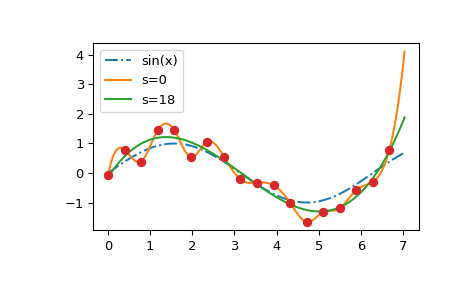
We now illustrate make_splrep results, using the same toy dataset as in the previous section

>>> import numpy as np
>>> from scipy.interpolate import make_splrep

Generate some noisy data

>>> x = np.arange(0, 2*np.pi+np.pi/4, 2*np.pi/16)
>>> rng = np.random.default_rng()
>>> y =  np.sin(x) + 0.4*rng.standard_normal(size=len(x))

Construct and plot smoothing splines for a series of values of the s parameter:

>>> import matplotlib.pyplot as plt
>>> xnew = np.arange(0, 9/4, 1/50) * np.pi

>>> plt.plot(xnew, np.sin(xnew), '-.', label='sin(x)')
>>> plt.plot(xnew, make_splrep(x, y, s=0)(xnew), '-', label='s=0')
>>> plt.plot(xnew, make_splrep(x, y, s=len(x))(xnew), '-', label=f's={len(x)}')
>>> plt.plot(x, y, 'o')
>>> plt.legend()
>>> plt.show()

We see that the \(s=0\) curve follows the (random) fluctuations of the data points, while the \(s > 0\) curve is close to the underlying sine function. Also note that the extrapolated values vary wildly depending on the value of \(s\).

Finding a good value of \(s\) is a trial-and-error process. If the weights correspond to the inverse of standard deviations of the input data, a “good” value of \(s\) is expected to be somewhere between \(m - \sqrt{2m}\) and \(m + \sqrt{2m}\), where \(m\) is the number of data points. If all weights equal unity, a reasonable choice might be around \(s \sim m\,\sigma^2\), where \(\sigma\) is an estimate for the standard deviation of the data.

Note

The number of knots is very strongly dependent on s. It is possible that small variations of s lead to drastic changes in the knot number.

Note

Both make_smoothing_spline and make_splrep allow for weighted fits, where the user provides an array of weights, w. Note that the definition differs somewhat: make_smoothing_spline squares the weights to be consistent with gcvspl, while make_splrep does not—to be consistent with FITPACK.

Effect of scaling the data

The smoothing condition is based on squared weighted residuals. Scaling y while keeping the same weights and s changes the effective smoothing strength. For example, multiplying y by 10 multiplies the residual sum of squares by 100 for a proportionally scaled fitted curve. As a result, the automatically selected knots and the shape of the fit need not be the same after rescaling.

The following comparison uses a fixed s and shows fitted curves after converting them back to the original data scale. In the right-hand plot, the weights are divided by the same positive scale factor as y. This preserves the weighted-residual constraint and makes the fits comparable across scales:

>>> import numpy as np
>>> import matplotlib.pyplot as plt
>>> from scipy.interpolate import make_splrep
>>> x = np.linspace(0, 2 * np.pi, 24)
>>> rng = np.random.default_rng(12345)
>>> y = np.sin(x) + 0.15 * rng.standard_normal(x.size)
>>> xnew = np.linspace(x[0], x[-1], 200)
>>> s = 0.35
>>> fig, axes = plt.subplots(1, 2, figsize=(10, 4), sharey=True)
>>> for scale in (0.1, 1, 10):
...     unweighted = make_splrep(x, scale * y, s=s)
...     weighted = make_splrep(x, scale * y,
...                            w=np.ones_like(x) / scale, s=s)
...     axes[0].plot(xnew, unweighted(xnew) / scale, label=f'scale={scale}')
...     axes[1].plot(xnew, weighted(xnew) / scale, label=f'scale={scale}')
>>> for ax in axes:
...     ax.plot(x, y, 'k.', alpha=0.45)
...     ax.legend()
>>> axes[0].set_title('Fixed weights and s')
>>> axes[1].set_title('Weights adjusted for scale')
>>> plt.tight_layout()
>>> plt.show()

For a positive scale factor \(a\), using w / a together with a * y keeps the squared weighted residuals unchanged when the fit is scaled by \(a\). This is one way to retain comparable smoothing when changing units. Alternatively, with fixed weights, scale s by \(a^2\). These transformations do not determine an optimal s for a new dataset; use weights reflecting measurement uncertainty when known.

Smoothing spline curves in \(d>1\)

So far we considered constructing smoothing spline functions, \(g(x)\) given data arrays x and y. We now consider a related problem of constructing a smoothing spline curve, where we consider the data as points on a plane, \(\mathbf{p}_j = (x_j, y_j)\), and we want to construct a parametric function \(\mathbf{g}(\mathbf{p}) = (g_x(u), g_y(u))\), where the values of the parameter \(u_j\) correspond to \(x_j\) and \(y_j\).

Note that this problem readily generalizes to higher dimensions, \(d > 2\): we simply have \(d\) data arrays and construct a parametric function with \(d\) components.

Also note that the choice of parametrization cannot be automated, and different parameterizations can lead to very different curves for the same data, even for interpolating curves.

Once a specific form of parametrization is chosen, the problem of constructing a smoothing curve is conceptually very similar to constructing a smoothing spline function. In a nutshell,

• spline knots are added from the values of the parameter \(u\), and

• both the cost function to minimize and the constraint we considered for spline functions simply get an extra summation over the \(d\) components.

The “parametric” generalization of the make_splrep function is make_splprep, and its docstring spells out the precise mathematical formulation of the minimization problem it solves.

The main user-visible difference of the parametric case is the user interface:

• instead of two data arrays, x and y, make_splprep receives a single two-dimensional array, where the first dimension has size \(d\) and each data array is stored along the second dimension (alternatively, you can supply a list of 1D arrays).

• the return value is pair: a BSpline instance and the array of parameter values, u, which corresponds to the input data arrays.

By default, make_splprep constructs and returns the chord length parametrization of input data (see the Parametric spline curves section for details). Alternatively, you can provide your own array of parameter values, u.

To illustrate the API, consider a toy problem: we have some data sampled from a folium of Descartes plus some noise.

>>> import numpy as np
>>> from scipy.interpolate import make_splprep
>>> th = np.linspace(-0.2, np.pi/2 + 0.2, 21)
>>> r = 3 * np.sin(th) * np.cos(th) / (np.sin(th)**3 + np.cos(th)**3)
>>> x, y = r * np.cos(th), r * np.sin(th)

Add some noise and construct the interpolators

>>> rng = np.random.default_rng()
>>> xn = x + 0.1*rng.uniform(-1, 1, size=len(x))
>>> yn = y + 0.1*rng.uniform(-1, 1, size=len(x))
>>> spl, u = make_splprep([xn, yn], s=0)   # note the [xn, yn] argument
>>> spl_n, u_n = make_splprep([xn, yn], s=0.1)

And plot the results (the result of spl(u) is a 2D array, so we unpack it into a pair of x and y arrays for plotting).

>>> import matplotlib.pyplot as plt
>>> plt.plot(xn, yn, 'o')
>>> plt.plot(*spl(u), '--')
>>> plt.plot(*spl_n(u_n), '-')
>>> plt.show()

Batching of y arrays

Unlike interpolating splines and GCV smoothers, make_splrep and make_splprep do not allow multidimensional y arrays and require that x.ndim == y.ndim == 1.

The technical reason for this limitation is that the length of the knot vector t depends on the y values, thus for a batched y, the batched t could be a ragged array, which BSpline is not equipped to handle.

Therefore if you need to handle batched inputs, you will need to loop over the batch manually and construct a BSpline object per slice of the batch. Having done that, you can mimic BSpline behavior for evaluations with a workaround along the lines of

class BatchSpline:
    """BSpline-like class with batch behavior."""
    def __init__(self, x, y, axis, *, spline, **kwargs):
        y = np.moveaxis(y, axis, -1)
        self._batch_shape = y.shape[:-1]
        self._splines = [
            spline(x, yi, **kwargs) for yi in y.reshape(-1, y.shape[-1])
        ]
        self._axis = axis

    def __call__(self, x):
        y = [spline(x) for spline in self._splines]
        y = np.reshape(y, self._batch_shape + x.shape)
        return np.moveaxis(y, -1, self._axis) if x.shape else y

Legacy routines for spline smoothing in 1-D

In addition to smoothing splines constructors we discussed in the previous sections, scipy.interpolate provides direct interfaces for routines from the venerable FITPACK Fortran library authored by P. Dierckx.

Note

These interfaces should be considered legacy—while we do not plan to deprecate or remove them, we recommend that new code uses more modern alternatives, make_smoothing_spline, make_splrep or make_splprep, instead.

For historical reasons, scipy.interpolate provides two equivalent interfaces for FITPACK, an interface and an object-oriented interface. While equivalent, these interfaces have different defaults. Below we discuss them in turn, starting from the functional interface.

Procedural (splrep)

Spline interpolation requires two essential steps: (1) a spline representation of the curve is computed, and (2) the spline is evaluated at the desired points. In order to find the spline representation, there are two different ways to represent a curve and obtain (smoothing) spline coefficients: directly and parametrically. The direct method finds the spline representation of a curve in a 2-D plane using the function splrep. The first two arguments are the only ones required, and these provide the \(x\) and \(y\) components of the curve. The normal output is a 3-tuple, \(\left(t,c,k\right)\) , containing the knot-points, \(t\) , the coefficients \(c\) and the order \(k\) of the spline. The default spline order is cubic, but this can be changed with the input keyword, k.

The knot array defines the interpolation interval to be t[k:-k], so that the first \(k+1\) and last \(k+1\) entries of the t array define boundary knots. The coefficients are a 1D array of length at least len(t) - k - 1. Some routines pad this array to have len(c) == len(t)— these additional coefficients are ignored for the spline evaluation.

The tck-tuple format is compatible with interpolating b-splines: the output of splrep can be wrapped into a BSpline object, e.g. BSpline(*tck), and the evaluation/integration/root-finding routines described below can use tck-tuples and BSpline objects interchangeably.

For curves in N-D space the function splprep allows defining the curve parametrically. For this function only 1 input argument is required. This input is a list of \(N\) arrays representing the curve in N-D space. The length of each array is the number of curve points, and each array provides one component of the N-D data point. The parameter variable is given with the keyword argument, u, which defaults to an equally-spaced monotonic sequence between \(0\) and \(1\) (i.e., the uniform parametrization).

The output consists of two objects: a 3-tuple, \(\left(t,c,k\right)\) , containing the spline representation and the parameter variable \(u.\)

The coefficients are a list of \(N\) arrays, where each array corresponds to a dimension of the input data. Note that the knots, t correspond to the parametrization of the curve u.

The keyword argument, s , is used to specify the amount of smoothing to perform during the spline fit. The default value of \(s\) is \(s=m-\sqrt{2m}\) where \(m\) is the number of data points being fit. Therefore, if no smoothing is desired a value of \(\mathbf{s}=0\) should be passed to the routines.

Once the spline representation of the data has been determined, it can be evaluated either using the splev function or by wrapping the tck tuple into a BSpline object, as demonstrated below.

We start by illustrating the effect of the s parameter on smoothing some synthetic noisy data

>>> import numpy as np
>>> from scipy.interpolate import splrep, BSpline

Generate some noisy data

>>> x = np.arange(0, 2*np.pi+np.pi/4, 2*np.pi/16)
>>> rng = np.random.default_rng()
>>> y =  np.sin(x) + 0.4*rng.standard_normal(size=len(x))

Construct two splines with different values of s.

>>> tck = splrep(x, y, s=0)
>>> tck_s = splrep(x, y, s=len(x))

And plot them

>>> import matplotlib.pyplot as plt
>>> xnew = np.arange(0, 9/4, 1/50) * np.pi
>>> plt.plot(xnew, np.sin(xnew), '-.', label='sin(x)')
>>> plt.plot(xnew, BSpline(*tck)(xnew), '-', label='s=0')
>>> plt.plot(xnew, BSpline(*tck_s)(xnew), '-', label=f's={len(x)}')
>>> plt.plot(x, y, 'o')
>>> plt.legend()
>>> plt.show()

We see that the s=0 curve follows the (random) fluctuations of the data points, while the s > 0 curve is close to the underlying sine function. Also note that the extrapolated values vary wildly depending on the value of s.

The default value of s depends on whether the weights are supplied or not, and also differs for splrep and splprep. Therefore, we recommend always providing the value of s explicitly.

Manipulating spline objects: procedural (splXXX)

Once the spline representation of the data has been determined, functions are available for evaluating the spline (splev) and its derivatives (splev, spalde) at any point and the integral of the spline between any two points ( splint). In addition, for cubic splines ( \(k=3\) ) with 8 or more knots, the roots of the spline can be estimated ( sproot). These functions are demonstrated in the example that follows.

>>> import numpy as np
>>> import matplotlib.pyplot as plt
>>> from scipy import interpolate

Cubic spline

>>> x = np.arange(0, 2*np.pi+np.pi/4, 2*np.pi/8)
>>> y = np.sin(x)
>>> tck = interpolate.splrep(x, y, s=0)
>>> xnew = np.arange(0, 2*np.pi, np.pi/50)
>>> ynew = interpolate.splev(xnew, tck, der=0)

Note that the last line is equivalent to BSpline(*tck)(xnew).

>>> plt.figure()
>>> plt.plot(x, y, 'x', xnew, ynew, xnew, np.sin(xnew), x, y, 'b')
>>> plt.legend(['Linear', 'Cubic Spline', 'True'])
>>> plt.axis([-0.05, 6.33, -1.05, 1.05])
>>> plt.title('Cubic-spline interpolation')
>>> plt.show()

Derivative of spline

>>> yder = interpolate.splev(xnew, tck, der=1)   # or BSpline(*tck)(xnew, 1)
>>> plt.figure()
>>> plt.plot(xnew, yder, xnew, np.cos(xnew),'--')
>>> plt.legend(['Cubic Spline', 'True'])
>>> plt.axis([-0.05, 6.33, -1.05, 1.05])
>>> plt.title('Derivative estimation from spline')
>>> plt.show()

All derivatives of spline

>>> yders = interpolate.spalde(xnew, tck)
>>> plt.figure()
>>> for i in range(len(yders[0])):
...    plt.plot(xnew, [d[i] for d in yders], '--', label=f"{i} derivative")
>>> plt.legend()
>>> plt.axis([-0.05, 6.33, -1.05, 1.05])
>>> plt.title('All derivatives of a B-spline')
>>> plt.show()

Integral of spline

>>> def integ(x, tck, constant=-1):
...     x = np.atleast_1d(x)
...     out = np.zeros(x.shape, dtype=x.dtype)
...     for n in range(len(out)):
...         out[n] = interpolate.splint(0, x[n], tck)
...     out += constant
...     return out

>>> yint = integ(xnew, tck)
>>> plt.figure()
>>> plt.plot(xnew, yint, xnew, -np.cos(xnew), '--')
>>> plt.legend(['Cubic Spline', 'True'])
>>> plt.axis([-0.05, 6.33, -1.05, 1.05])
>>> plt.title('Integral estimation from spline')
>>> plt.show()

Roots of spline

>>> interpolate.sproot(tck)
array([3.1416])  # may vary

Notice that sproot may fail to find an obvious solution at the edge of the approximation interval, \(x = 0\). If we define the spline on a slightly larger interval, we recover both roots \(x = 0\) and \(x = \pi\):

>>> x = np.linspace(-np.pi/4, np.pi + np.pi/4, 51)
>>> y = np.sin(x)
>>> tck = interpolate.splrep(x, y, s=0)
>>> interpolate.sproot(tck)
array([0., 3.1416])

Parametric spline

>>> t = np.arange(0, 1.1, .1)
>>> x = np.sin(2*np.pi*t)
>>> y = np.cos(2*np.pi*t)
>>> tck, u = interpolate.splprep([x, y], s=0)
>>> unew = np.arange(0, 1.01, 0.01)
>>> out = interpolate.splev(unew, tck)
>>> plt.figure()
>>> plt.plot(x, y, 'x', out[0], out[1], np.sin(2*np.pi*unew), np.cos(2*np.pi*unew), x, y, 'b')
>>> plt.legend(['Linear', 'Cubic Spline', 'True'])
>>> plt.axis([-1.05, 1.05, -1.05, 1.05])
>>> plt.title('Spline of parametrically-defined curve')
>>> plt.show()

Note that in the last example, splprep returns the spline coefficients as a list of arrays, where each array corresponds to a dimension of the input data. Thus to wrap its output to a BSpline, we need to transpose the coefficients (or use BSpline(..., axis=1)):

>>> tt, cc, k = tck
>>> cc = np.array(cc)
>>> bspl = BSpline(tt, cc.T, k)    # note the transpose
>>> xy = bspl(u)
>>> xx, yy = xy.T   # transpose to unpack into a pair of arrays
>>> np.allclose(x, xx)
True
>>> np.allclose(y, yy)
True

Object-oriented (UnivariateSpline)

The spline-fitting capabilities described above are also available via an objected-oriented interface. The 1-D splines are objects of the UnivariateSpline class, and are created with the \(x\) and \(y\) components of the curve provided as arguments to the constructor. The class defines __call__, allowing the object to be called with the x-axis values, at which the spline should be evaluated, returning the interpolated y-values. This is shown in the example below for the subclass InterpolatedUnivariateSpline. The integral, derivatives, and roots methods are also available on UnivariateSpline objects, allowing definite integrals, derivatives, and roots to be computed for the spline.

The UnivariateSpline class can also be used to smooth data by providing a non-zero value of the smoothing parameter s, with the same meaning as the s keyword of the splrep function described above. This results in a spline that has fewer knots than the number of data points, and hence is no longer strictly an interpolating spline, but rather a smoothing spline. If this is not desired, the InterpolatedUnivariateSpline class is available. It is a subclass of UnivariateSpline that always passes through all points (equivalent to forcing the smoothing parameter to 0). This class is demonstrated in the example below.

The LSQUnivariateSpline class is the other subclass of UnivariateSpline. It allows the user to specify the number and location of internal knots explicitly with the parameter t. This allows for the creation of customized splines with non-linear spacing, to interpolate in some domains and smooth in others, or change the character of the spline.

>>> import numpy as np
>>> import matplotlib.pyplot as plt
>>> from scipy import interpolate

InterpolatedUnivariateSpline

>>> x = np.arange(0, 2*np.pi+np.pi/4, 2*np.pi/8)
>>> y = np.sin(x)
>>> s = interpolate.InterpolatedUnivariateSpline(x, y)
>>> xnew = np.arange(0, 2*np.pi, np.pi/50)
>>> ynew = s(xnew)

>>> plt.figure()
>>> plt.plot(x, y, 'x', xnew, ynew, xnew, np.sin(xnew), x, y, 'b')
>>> plt.legend(['Linear', 'InterpolatedUnivariateSpline', 'True'])
>>> plt.axis([-0.05, 6.33, -1.05, 1.05])
>>> plt.title('InterpolatedUnivariateSpline')
>>> plt.show()

LSQUnivarateSpline with non-uniform knots

>>> t = [np.pi/2-.1, np.pi/2+.1, 3*np.pi/2-.1, 3*np.pi/2+.1]
>>> s = interpolate.LSQUnivariateSpline(x, y, t, k=2)
>>> ynew = s(xnew)

>>> plt.figure()
>>> plt.plot(x, y, 'x', xnew, ynew, xnew, np.sin(xnew), x, y, 'b')
>>> plt.legend(['Linear', 'LSQUnivariateSpline', 'True'])
>>> plt.axis([-0.05, 6.33, -1.05, 1.05])
>>> plt.title('Spline with Specified Interior Knots')
>>> plt.show()

2-D smoothing splines

In addition to smoothing 1-D splines, the FITPACK library provides the means of fitting 2-D surfaces to two-dimensional data. The surfaces can be thought of as functions of two arguments, \(z = g(x, y)\), constructed as tensor products of 1-D splines.

Assuming that the data is held in three arrays, x, y and z, there are two ways these data arrays can be interpreted. First—the scattered interpolation problem—the data is assumed to be paired, i.e. the pairs of values x[i] and y[i] represent the coordinates of the point i, which corresponds to z[i].

The surface \(g(x, y)\) is constructed to satisfy

\[\sum_i \left[ w_i (g(x_i, y_i) - z_i)\right]^2 \leqslant s\]

where \(w_i\) are non-negative weights, and s is the input parameter, known as the smoothing factor, which controls the interplay between smoothness of the resulting function g(x, y) and the quality of the approximation of the data (i.e., the differences between \(g(x_i, y_i)\) and \(z_i\)). The limit of \(s = 0\) formally corresponds to interpolation, where the surface passes through the input data, \(g(x_i, y_i) = z_i\). See the note below however.

The second case—the rectangular grid interpolation problem—is where the data points are assumed to be on a rectangular grid defined by all pairs of the elements of the x and y arrays. For this problem, the z array is assumed to be two-dimensional, and z[i, j] corresponds to (x[i], y[j]). The bivariate spline function \(g(x, y)\) is constructed to satisfy

\[\sum_i \sum_j \left[ (g(x_i, y_j) - z_{i,j})\right]^2 \leqslant s\]

where s is the smoothing factor. Here the limit of \(s=0\) also formally corresponds to interpolation, \(g(x_i, y_j) = z_{i, j}\).

Note

Internally, the smoothing surface \(g(x, y)\) is constructed by placing spline knots into the bounding box defined by the data arrays. The knots are placed automatically via the FITPACK algorithm until the desired smoothness is reached.

The knots may be placed away from the data points.

While \(s=0\) formally corresponds to a bivariate spline interpolation, the FITPACK algorithm is not meant for interpolation, and may lead to unexpected results.

For scattered data interpolation, prefer griddata; for data on a regular grid, prefer RegularGridInterpolator.

Note

If the input data, x and y, is such that input dimensions have incommensurate units and differ by many orders of magnitude, the interpolant \(g(x, y)\) may have numerical artifacts. Consider rescaling the data before interpolation.

We now consider the two spline fitting problems in turn.

Bivariate spline fitting of scattered data

There are two interfaces for the underlying FITPACK library, a procedural one and an object-oriented interface.

Procedural interface (`bisplrep`)

For (smooth) spline fitting to a 2-D surface, the function bisplrep is available. This function takes as required inputs the 1-D arrays x, y, and z, which represent points on the surface \(z=f(x, y).\) The spline orders in x and y directions can be specified via the optional parameters kx and ky. The default is a bicubic spline, kx=ky=3.

The output of bisplrep is a list [tx ,ty, c, kx, ky] whose entries represent respectively, the components of the knot positions, the coefficients of the spline, and the order of the spline in each coordinate. It is convenient to hold this list in a single object, tck, so that it can be passed easily to the function bisplev. The keyword, s , can be used to change the amount of smoothing performed on the data while determining the appropriate spline. The recommended values for \(s\) depend on the weights \(w_i\). If these are taken as \(1/d_i\), with \(d_i\) an estimate of the standard deviation of \(z_i\), a good value of \(s\) should be found in the range \(m- \sqrt{2m}, m + \sqrt{2m}\), where \(m\) is the number of data points in the x, y, and z vectors.

The default value is \(s=m-\sqrt{2m}\). As a result, if no smoothing is desired, then ``s=0`` should be passed to `bisplrep`. (See however the note above).

To evaluate the 2-D spline and its partial derivatives (up to the order of the spline), the function bisplev is required. This function takes as the first two arguments two 1-D arrays whose cross-product specifies the domain over which to evaluate the spline. The third argument is the tck list returned from bisplrep. If desired, the fourth and fifth arguments provide the orders of the partial derivative in the \(x\) and \(y\) direction, respectively.

Note

It is important to note that 2-D interpolation should not be used to find the spline representation of images. The algorithm used is not amenable to large numbers of input points. scipy.signal and scipy.ndimage contain more appropriate algorithms for finding the spline representation of an image.

The 2-D interpolation commands are intended for use when interpolating a 2-D function as shown in the example that follows. This example uses the mgrid command in NumPy which is useful for defining a “mesh-grid” in many dimensions. (See also the ogrid command if the full-mesh is not needed). The number of output arguments and the number of dimensions of each argument is determined by the number of indexing objects passed in mgrid.

>>> import numpy as np
>>> from scipy import interpolate
>>> import matplotlib.pyplot as plt

Define function over a sparse 20x20 grid

>>> x_edges, y_edges = np.mgrid[-1:1:21j, -1:1:21j]
>>> x = x_edges[:-1, :-1] + np.diff(x_edges[:2, 0])[0] / 2.
>>> y = y_edges[:-1, :-1] + np.diff(y_edges[0, :2])[0] / 2.
>>> z = (x+y) * np.exp(-6.0*(x*x+y*y))

>>> plt.figure()
>>> lims = dict(cmap='RdBu_r', vmin=-0.25, vmax=0.25)
>>> plt.pcolormesh(x_edges, y_edges, z, shading='flat', **lims)
>>> plt.colorbar()
>>> plt.title("Sparsely sampled function.")
>>> plt.show()

Interpolate function over a new 70x70 grid

>>> xnew_edges, ynew_edges = np.mgrid[-1:1:71j, -1:1:71j]
>>> xnew = xnew_edges[:-1, :-1] + np.diff(xnew_edges[:2, 0])[0] / 2.
>>> ynew = ynew_edges[:-1, :-1] + np.diff(ynew_edges[0, :2])[0] / 2.
>>> tck = interpolate.bisplrep(x, y, z, s=0)
>>> znew = interpolate.bisplev(xnew[:,0], ynew[0,:], tck)

>>> plt.figure()
>>> plt.pcolormesh(xnew_edges, ynew_edges, znew, shading='flat', **lims)
>>> plt.colorbar()
>>> plt.title("Interpolated function.")
>>> plt.show()

Object-oriented interface (`SmoothBivariateSpline`)

The object-oriented interface for bivariate spline smoothing of scattered data, SmoothBivariateSpline class, implements a subset of the functionality of the bisplrep / bisplev pair, and has different defaults.

It takes the elements of the weights array equal unity, \(w_i = 1\) and constructs the knot vectors automatically given the input value of the smoothing factor s— the default value is \(m\), the number of data points.

The spline orders in the x and y directions are controlled by the optional parameters kx and ky, with the default of kx=ky=3.

We illustrate the effect of the smoothing factor using the following example:

import numpy as np
import matplotlib.pyplot as plt
from scipy.interpolate import SmoothBivariateSpline

import warnings
warnings.simplefilter('ignore')

train_x, train_y = np.meshgrid(np.arange(-5, 5, 0.5), np.arange(-5, 5, 0.5))
train_x = train_x.flatten()
train_y = train_y.flatten()

def z_func(x, y):
    return np.cos(x) + np.sin(y) ** 2 + 0.05 * x + 0.1 * y

train_z = z_func(train_x, train_y)
interp_func = SmoothBivariateSpline(train_x, train_y, train_z, s=0.0)
smth_func = SmoothBivariateSpline(train_x, train_y, train_z)

test_x = np.arange(-9, 9, 0.01)
test_y = np.arange(-9, 9, 0.01)
grid_x, grid_y = np.meshgrid(test_x, test_y)

interp_result = interp_func(test_x, test_y).T
smth_result = smth_func(test_x, test_y).T
perfect_result = z_func(grid_x, grid_y)

fig, axes = plt.subplots(1, 3, figsize=(16, 8))
extent = [test_x[0], test_x[-1], test_y[0], test_y[-1]]
opts = dict(aspect='equal', cmap='nipy_spectral', extent=extent, vmin=-1.5, vmax=2.5)

im = axes[0].imshow(perfect_result, **opts)
fig.colorbar(im, ax=axes[0], orientation='horizontal')
axes[0].plot(train_x, train_y, 'w.')
axes[0].set_title('Perfect result, sampled function', fontsize=21)

im = axes[1].imshow(smth_result, **opts)
axes[1].plot(train_x, train_y, 'w.')
fig.colorbar(im, ax=axes[1], orientation='horizontal')
axes[1].set_title('s=default', fontsize=21)

im = axes[2].imshow(interp_result, **opts)
fig.colorbar(im, ax=axes[2], orientation='horizontal')
axes[2].plot(train_x, train_y, 'w.')
axes[2].set_title('s=0', fontsize=21)

plt.tight_layout()
plt.show()

Here we take a known function (displayed at the leftmost panel), sample it on a mesh of points (shown by white dots), and construct the spline fit using the default smoothing (center panel) and forcing the interpolation (rightmost panel).

Several features are clearly visible. First, the default value of s provides too much smoothing for this data; forcing the interpolation condition, s = 0, allows to restore the underlying function to a reasonable accuracy. Second, outside of the interpolation range (i.e., the area covered by white dots) the result is extrapolated using a nearest-neighbor constant. Finally, we had to silence the warnings (which is a bad form, yes!).

The warning here is emitted in the s=0 case, and signals an internal difficulty FITPACK encountered when we forced the interpolation condition. If you see this warning in your code, consider switching to bisplrep and increase its nxest, nyest parameters (see the bisplrep docstring for more details).

Bivariate spline fitting of data on a grid

For gridded 2D data, fitting a smoothing tensor product spline can be done using the RectBivariateSpline class. It has the interface similar to that of SmoothBivariateSpline, the main difference is that the 1D input arrays x and y are understood as defining a 2D grid (as their outer product), and the z array is 2D with the shape of len(x) by len(y).

The spline orders in the x and y directions are controlled by the optional parameters kx and ky, with the default of kx=ky=3, i.e. a bicubic spline.

The default value of the smoothing factor is s=0. We nevertheless recommend to always specify s explicitly.

import numpy as np
import matplotlib.pyplot as plt
from scipy.interpolate import RectBivariateSpline

x = np.arange(-5.01, 5.01, 0.25)        # the grid is an outer product
y = np.arange(-5.01, 7.51, 0.25)        # of x and y arrays

xx, yy = np.meshgrid(x, y, indexing='ij')
z = np.sin(xx**2 + 2.*yy**2)            # z array needs to be 2-D

func = RectBivariateSpline(x, y, z, s=0)

xnew = np.arange(-5.01, 5.01, 1e-2)
ynew = np.arange(-5.01, 7.51, 1e-2)
znew = func(xnew, ynew)

plt.imshow(znew)
plt.colorbar()
plt.show()

Bivariate spline fitting of data in spherical coordinates

If your data is given in spherical coordinates, \(r = r(\theta, \phi)\), SmoothSphereBivariateSpline and RectSphereBivariateSpline provide convenient analogs of SmoothBivariateSpline and RectBivariateSpline, respectively.

These classes ensure the periodicity of the spline fits for \(\theta \in [0, \pi]\) and \(\phi \in [0, 2\pi]\), and offer some control over the continuity at the poles. Refer to the docstrings of these classes for details.