scipy.stats.nchypergeom_fisher#

scipy.stats.nchypergeom_fisher = <scipy.stats._discrete_distns.nchypergeom_fisher_gen object>[source]#

A Fisher’s noncentral hypergeometric discrete random variable.

Fisher’s noncentral hypergeometric distribution models drawing objects of two types from a bin. M is the total number of objects, n is the number of Type I objects, and odds is the odds ratio: the odds of selecting a Type I object rather than a Type II object when there is only one object of each type. The random variate represents the number of Type I objects drawn if we take a handful of objects from the bin at once and find out afterwards that we took N objects.

As an instance of the rv_discrete class, nchypergeom_fisher object inherits from it a collection of generic methods (see below for the full list), and completes them with details specific for this particular distribution.

See also

nchypergeom_wallenius, hypergeom, nhypergeom

Notes

Let mathematical symbols \(N\), \(n\), and \(M\) correspond with parameters N, n, and M (respectively) as defined above.

The probability mass function is defined as

\[p(x; M, n, N, \omega) = \frac{\binom{n}{x}\binom{M - n}{N-x}\omega^x}{P_0},\]

for \(x \in [x_l, x_u]\), \(M \in {\mathbb N}\), \(n \in [0, M]\), \(N \in [0, M]\), \(\omega > 0\), where \(x_l = \max(0, N - (M - n))\), \(x_u = \min(N, n)\),

\[P_0 = \sum_{y=x_l}^{x_u} \binom{n}{y}\binom{M - n}{N-y}\omega^y,\]

and the binomial coefficients are defined as

\[\binom{n}{k} \equiv \frac{n!}{k! (n - k)!}.\]

nchypergeom_fisher uses the BiasedUrn package by Agner Fog with permission for it to be distributed under SciPy’s license.

The symbols used to denote the shape parameters (N, n, and M) are not universally accepted; they are chosen for consistency with hypergeom.

Note that Fisher’s noncentral hypergeometric distribution is distinct from Wallenius’ noncentral hypergeometric distribution, which models drawing a pre-determined N objects from a bin one by one. When the odds ratio is unity, however, both distributions reduce to the ordinary hypergeometric distribution.

The probability mass function above is defined in the “standardized” form. To shift distribution use the loc parameter. Specifically, nchypergeom_fisher.pmf(k, M, n, N, odds, loc) is identically equivalent to nchypergeom_fisher.pmf(k - loc, M, n, N, odds).

References

[1]

Agner Fog, “Biased Urn Theory”. https://cran.r-project.org/web/packages/BiasedUrn/vignettes/UrnTheory.pdf

[2]

“Fisher’s noncentral hypergeometric distribution”, Wikipedia, https://en.wikipedia.org/wiki/Fisher’s_noncentral_hypergeometric_distribution

Examples

>>> import numpy as np
>>> from scipy.stats import nchypergeom_fisher
>>> import matplotlib.pyplot as plt
>>> fig, ax = plt.subplots(1, 1)

Calculate the first four moments:

>>> M, n, N, odds = 140, 80, 60, 0.5
>>> mean, var, skew, kurt = nchypergeom_fisher.stats(M, n, N, odds, moments='mvsk')

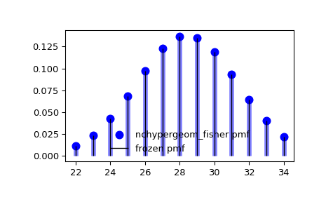
Display the probability mass function (pmf):

>>> x = np.arange(nchypergeom_fisher.ppf(0.01, M, n, N, odds),
...               nchypergeom_fisher.ppf(0.99, M, n, N, odds))
>>> ax.plot(x, nchypergeom_fisher.pmf(x, M, n, N, odds), 'bo', ms=8, label='nchypergeom_fisher pmf')
>>> ax.vlines(x, 0, nchypergeom_fisher.pmf(x, M, n, N, odds), colors='b', lw=5, alpha=0.5)

Alternatively, the distribution object can be called (as a function) to fix the shape and location. This returns a “frozen” RV object holding the given parameters fixed.

Freeze the distribution and display the frozen pmf:

>>> rv = nchypergeom_fisher(M, n, N, odds)
>>> ax.vlines(x, 0, rv.pmf(x), colors='k', linestyles='-', lw=1,
...         label='frozen pmf')
>>> ax.legend(loc='best', frameon=False)
>>> plt.show()

../../_images/scipy-stats-nchypergeom_fisher-1_00_00.png

Check accuracy of cdf and ppf:

>>> prob = nchypergeom_fisher.cdf(x, M, n, N, odds)
>>> np.allclose(x, nchypergeom_fisher.ppf(prob, M, n, N, odds))
True

Generate random numbers:

>>> r = nchypergeom_fisher.rvs(M, n, N, odds, size=1000)

Methods

rvs(M, n, N, odds, loc=0, size=1, random_state=None)	Random variates.
pmf(k, M, n, N, odds, loc=0)	Probability mass function.
logpmf(k, M, n, N, odds, loc=0)	Log of the probability mass function.
cdf(k, M, n, N, odds, loc=0)	Cumulative distribution function.
logcdf(k, M, n, N, odds, loc=0)	Log of the cumulative distribution function.
sf(k, M, n, N, odds, loc=0)	Survival function (also defined as `1 - cdf`, but sf is sometimes more accurate).
logsf(k, M, n, N, odds, loc=0)	Log of the survival function.
ppf(q, M, n, N, odds, loc=0)	Percent point function (inverse of `cdf` — percentiles).
isf(q, M, n, N, odds, loc=0)	Inverse survival function (inverse of `sf`).
stats(M, n, N, odds, loc=0, moments=’mv’)	Mean(‘m’), variance(‘v’), skew(‘s’), and/or kurtosis(‘k’).
entropy(M, n, N, odds, loc=0)	(Differential) entropy of the RV.
expect(func, args=(M, n, N, odds), loc=0, lb=None, ub=None, conditional=False)	Expected value of a function (of one argument) with respect to the distribution.
median(M, n, N, odds, loc=0)	Median of the distribution.
mean(M, n, N, odds, loc=0)	Mean of the distribution.
var(M, n, N, odds, loc=0)	Variance of the distribution.
std(M, n, N, odds, loc=0)	Standard deviation of the distribution.
interval(confidence, M, n, N, odds, loc=0)	Confidence interval with equal areas around the median.