scipy.stats.nbinom

scipy.stats.nbinom = <scipy.stats._discrete_distns.nbinom_gen object>

A negative binomial discrete random variable.

As an instance of the rv_discrete class, nbinom object inherits from it a collection of generic methods (see below for the full list), and completes them with details specific for this particular distribution.

See also

hypergeom, binom, nhypergeom

Notes

Negative binomial distribution describes a sequence of i.i.d. Bernoulli trials, repeated until a predefined, non-random number of successes occurs.

The probability mass function of the number of failures for nbinom is:

\[f(k) = \binom{k+n-1}{n-1} p^n (1-p)^k\]

for \(k \ge 0\), \(0 < p \leq 1\)

nbinom takes \(n\) and \(p\) as shape parameters where \(n\) is the number of successes, \(p\) is the probability of a single success, and \(1-p\) is the probability of a single failure.

Another common parameterization of the negative binomial distribution is in terms of the mean number of failures \(\mu\) to achieve \(n\) successes. The mean \(\mu\) is related to the probability of success as

\[p = \frac{n}{n + \mu}\]

The number of successes \(n\) may also be specified in terms of a “dispersion”, “heterogeneity”, or “aggregation” parameter \(\alpha\), which relates the mean \(\mu\) to the variance \(\sigma^2\), e.g. \(\sigma^2 = \mu + \alpha \mu^2\). Regardless of the convention used for \(\alpha\),

\[\begin{split}p &= \frac{\mu}{\sigma^2} \\ n &= \frac{\mu^2}{\sigma^2 - \mu}\end{split}\]

The probability mass function above is defined in the “standardized” form. To shift distribution use the loc parameter. Specifically, nbinom.pmf(k, n, p, loc) is identically equivalent to nbinom.pmf(k - loc, n, p).

Examples

Try it in your browser!

>>> import numpy as np
>>> from scipy.stats import nbinom
>>> import matplotlib.pyplot as plt
>>> fig, ax = plt.subplots(1, 1)

Calculate the first four moments:

>>> n, p = 5, 0.5
>>> mean, var, skew, kurt = nbinom.stats(n, p, moments='mvsk')

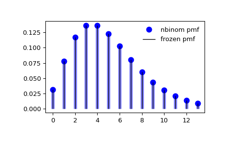
Display the probability mass function (pmf):

>>> x = np.arange(nbinom.ppf(0.01, n, p),
...               nbinom.ppf(0.99, n, p))
>>> ax.plot(x, nbinom.pmf(x, n, p), 'bo', ms=8, label='nbinom pmf')
>>> ax.vlines(x, 0, nbinom.pmf(x, n, p), colors='b', lw=5, alpha=0.5)

Alternatively, the distribution object can be called (as a function) to fix the shape and location. This returns a “frozen” RV object holding the given parameters fixed.

Freeze the distribution and display the frozen pmf:

>>> rv = nbinom(n, p)
>>> ax.vlines(x, 0, rv.pmf(x), colors='k', linestyles='-', lw=1,
...         label='frozen pmf')
>>> ax.legend(loc='best', frameon=False)
>>> plt.show()

Check accuracy of cdf and ppf:

>>> prob = nbinom.cdf(x, n, p)
>>> np.allclose(x, nbinom.ppf(prob, n, p))
True

Generate random numbers:

>>> r = nbinom.rvs(n, p, size=1000)

Go BackOpen In Tab

Methods

rvs(n, p, loc=0, size=1, random_state=None)	Random variates.
pmf(k, n, p, loc=0)	Probability mass function.
logpmf(k, n, p, loc=0)	Log of the probability mass function.
cdf(k, n, p, loc=0)	Cumulative distribution function.
logcdf(k, n, p, loc=0)	Log of the cumulative distribution function.
sf(k, n, p, loc=0)	Survival function (also defined as 1 - cdf, but sf is sometimes more accurate).
logsf(k, n, p, loc=0)	Log of the survival function.
ppf(q, n, p, loc=0)	Percent point function (inverse of cdf — percentiles).
isf(q, n, p, loc=0)	Inverse survival function (inverse of sf).
stats(n, p, loc=0, moments=’mv’)	Mean(‘m’), variance(‘v’), skew(‘s’), and/or kurtosis(‘k’).
entropy(n, p, loc=0)	(Differential) entropy of the RV.
expect(func, args=(n, p), loc=0, lb=None, ub=None, conditional=False)	Expected value of a function (of one argument) with respect to the distribution.
median(n, p, loc=0)	Median of the distribution.
mean(n, p, loc=0)	Mean of the distribution.
var(n, p, loc=0)	Variance of the distribution.
std(n, p, loc=0)	Standard deviation of the distribution.
interval(confidence, n, p, loc=0)	Confidence interval with equal areas around the median.