scipy.special.nbdtrik#

scipy.special.nbdtrik(y, n, p, out=None) = <ufunc 'nbdtrik'>#

Negative binomial percentile function.

Returns the inverse with respect to the parameter k of y = nbdtr(k, n, p), the negative binomial cumulative distribution function.

Parameters:

yarray_like: The probability of k or fewer failures before n successes (float).
narray_like: The target number of successes (positive int).
parray_like: Probability of success in a single event (float).
outndarray, optional: Optional output array for the function results

Returns:

kscalar or ndarray: The maximum number of allowed failures such that nbdtr(k, n, p) = y.

See also

nbdtr: Cumulative distribution function of the negative binomial.
nbdtrc: Survival function of the negative binomial.
nbdtri: Inverse with respect to p of nbdtr(k, n, p).
nbdtrin: Inverse with respect to n of nbdtr(k, n, p).
scipy.stats.nbinom: Negative binomial distribution

Notes

Wrapper for the CDFLIB [1] Fortran routine cdfnbn.

Formula 26.5.26 of [2],

\[\sum_{j=k + 1}^\infty {{n + j - 1} \choose{j}} p^n (1 - p)^j = I_{1 - p}(k + 1, n),\]

is used to reduce calculation of the cumulative distribution function to that of a regularized incomplete beta \(I\).

Computation of k involves a search for a value that produces the desired value of y. The search relies on the monotonicity of y with k.

References

[1]

Barry Brown, James Lovato, and Kathy Russell, CDFLIB: Library of Fortran Routines for Cumulative Distribution Functions, Inverses, and Other Parameters.

[2]

Milton Abramowitz and Irene A. Stegun, eds. Handbook of Mathematical Functions with Formulas, Graphs, and Mathematical Tables. New York: Dover, 1972.

Examples

Compute the negative binomial cumulative distribution function for an exemplary parameter set.

>>> import numpy as np
>>> from scipy.special import nbdtr, nbdtrik
>>> k, n, p = 5, 2, 0.5
>>> cdf_value = nbdtr(k, n, p)
>>> cdf_value
0.9375

Verify that nbdtrik recovers the original value for k.

>>> nbdtrik(cdf_value, n, p)
5.0

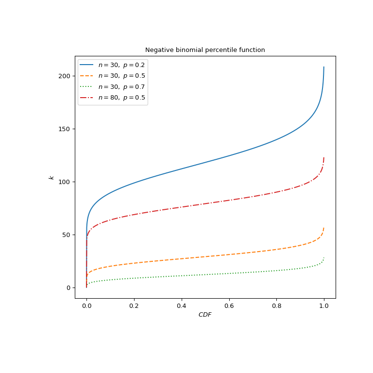
Plot the function for different parameter sets.

>>> import matplotlib.pyplot as plt
>>> p_parameters = [0.2, 0.5, 0.7, 0.5]
>>> n_parameters = [30, 30, 30, 80]
>>> linestyles = ['solid', 'dashed', 'dotted', 'dashdot']
>>> parameters_list = list(zip(p_parameters, n_parameters, linestyles))
>>> cdf_vals = np.linspace(0, 1, 1000)
>>> fig, ax = plt.subplots(figsize=(8, 8))
>>> for parameter_set in parameters_list:
...     p, n, style = parameter_set
...     nbdtrik_vals = nbdtrik(cdf_vals, n, p)
...     ax.plot(cdf_vals, nbdtrik_vals, label=rf"$n={n},\ p={p}$",
...             ls=style)
>>> ax.legend()
>>> ax.set_ylabel("$k$")
>>> ax.set_xlabel("$CDF$")
>>> ax.set_title("Negative binomial percentile function")
>>> plt.show()

../../_images/scipy-special-nbdtrik-1_00_00.png

The negative binomial distribution is also available as scipy.stats.nbinom. The percentile function method ppf returns the result of nbdtrik rounded up to integers:

>>> from scipy.stats import nbinom
>>> q, n, p = 0.6, 5, 0.5
>>> nbinom.ppf(q, n, p), nbdtrik(q, n, p)
(5.0, 4.800428460273882)