scipy.integrate.

cumulative_trapezoid#

scipy.integrate.cumulative_trapezoid(y, x=None, dx=1.0, axis=-1, initial=None)[source]#

Cumulatively integrate y(x) using the composite trapezoidal rule.

Parameters:

yarray_like: Values to integrate.
xarray_like, optional: The coordinate to integrate along. If None (default), use spacing dx between consecutive elements in y.
dxfloat, optional: Spacing between elements of y. Only used if x is None.
axisint, optional: Specifies the axis to cumulate. Default is -1 (last axis).
initialscalar, optional: If given, insert this value at the beginning of the returned result. 0 or None are the only values accepted. Default is None, which means res has one element less than y along the axis of integration.

Returns:

resndarray: The result of cumulative integration of y along axis. If initial is None, the shape is such that the axis of integration has one less value than y. If initial is given, the shape is equal to that of y.

See also

numpy.cumsum, numpy.cumprod
cumulative_simpson: cumulative integration using Simpson’s 1/3 rule
quad: adaptive quadrature using QUADPACK
fixed_quad: fixed-order Gaussian quadrature
dblquad: double integrals
tplquad: triple integrals
romb: integrators for sampled data

Notes

Array API Standard Support

cumulative_trapezoid has experimental support for Python Array API Standard compatible backends in addition to NumPy. Please consider testing these features by setting an environment variable SCIPY_ARRAY_API=1 and providing CuPy, PyTorch, JAX, or Dask arrays as array arguments. The following combinations of backend and device (or other capability) are supported.

Library	CPU	GPU
NumPy	✅	n/a
CuPy	n/a	✅
PyTorch	✅	✅
JAX	✅	✅
Dask	✅	n/a

See Support for the array API standard for more information.

Examples

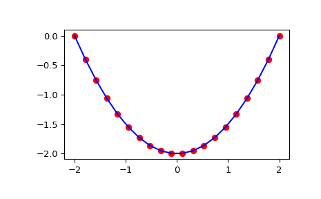
>>> from scipy import integrate
>>> import numpy as np
>>> import matplotlib.pyplot as plt

>>> x = np.linspace(-2, 2, num=20)
>>> y = x
>>> y_int = integrate.cumulative_trapezoid(y, x, initial=0)
>>> plt.plot(x, y_int, 'ro', x, y[0] + 0.5 * x**2, 'b-')
>>> plt.show()

../../_images/scipy-integrate-cumulative_trapezoid-1.png