cumulative_simpson#
- scipy.integrate.cumulative_simpson(y, *, x=None, dx=1.0, axis=-1, initial=None)[source]#
Cumulatively integrate y(x) using the composite Simpson’s 1/3 rule. The integral of the samples at every point is calculated by assuming a quadratic relationship between each point and the two adjacent points.
- Parameters:
- yarray_like
Values to integrate. Requires at least one point along axis. If two or fewer points are provided along axis, Simpson’s integration is not possible and the result is calculated with
cumulative_trapezoid.- xarray_like, optional
The coordinate to integrate along. Must have the same shape as y or must be 1D with the same length as y along axis. x must also be strictly increasing along axis. If x is None (default), integration is performed using spacing dx between consecutive elements in y.
- dxscalar or array_like, optional
Spacing between elements of y. Only used if x is None. Can either be a float, or an array with the same shape as y, but of length one along axis. Default is 1.0.
- axisint, optional
Specifies the axis to integrate along. Default is -1 (last axis).
- initialscalar or array_like, optional
If given, insert this value at the beginning of the returned result, and add it to the rest of the result. Default is None, which means no value at
x[0]is returned and res has one element less than y along the axis of integration. Can either be a float, or an array with the same shape as y, but of length one along axis.
- Returns:
- resndarray
The result of cumulative integration of y along axis. If initial is None, the shape is such that the axis of integration has one less value than y. If initial is given, the shape is equal to that of y.
See also
numpy.cumsumcumulative_trapezoidcumulative integration using the composite trapezoidal rule
simpsonintegrator for sampled data using the Composite Simpson’s Rule
Notes
Added in version 1.12.0.
The composite Simpson’s 1/3 method can be used to approximate the definite integral of a sampled input function \(y(x)\) [1]. The method assumes a quadratic relationship over the interval containing any three consecutive sampled points.
Consider three consecutive points: \((x_1, y_1), (x_2, y_2), (x_3, y_3)\).
Assuming a quadratic relationship over the three points, the integral over the subinterval between \(x_1\) and \(x_2\) is given by formula (8) of [2]:
\[\begin{split}\int_{x_1}^{x_2} y(x) dx\ &= \frac{x_2-x_1}{6}\left[\ \left\{3-\frac{x_2-x_1}{x_3-x_1}\right\} y_1 + \ \left\{3 + \frac{(x_2-x_1)^2}{(x_3-x_2)(x_3-x_1)} + \ \frac{x_2-x_1}{x_3-x_1}\right\} y_2\\ - \frac{(x_2-x_1)^2}{(x_3-x_2)(x_3-x_1)} y_3\right]\end{split}\]The integral between \(x_2\) and \(x_3\) is given by swapping appearances of \(x_1\) and \(x_3\). The integral is estimated separately for each subinterval and then cumulatively summed to obtain the final result.
For samples that are equally spaced, the result is exact if the function is a polynomial of order three or less [1] and the number of subintervals is even. Otherwise, the integral is exact for polynomials of order two or less.
Array API Standard Support
cumulative_simpsonhas experimental support for Python Array API Standard compatible backends in addition to NumPy. Please consider testing these features by setting an environment variableSCIPY_ARRAY_API=1and providing CuPy, PyTorch, JAX, or Dask arrays as array arguments. The following combinations of backend and device (or other capability) are supported.Library
CPU
GPU
NumPy
✅
n/a
CuPy
n/a
✅
PyTorch
✅
✅
JAX
⛔
⛔
Dask
⚠️ computes graph
n/a
See Support for the array API standard for more information.
References
[2]Cartwright, Kenneth V. Simpson’s Rule Cumulative Integration with MS Excel and Irregularly-spaced Data. Journal of Mathematical Sciences and Mathematics Education. 12 (2): 1-9
Examples
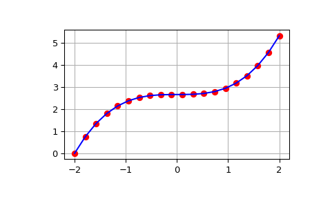
>>> from scipy import integrate
>>> import numpy as np
>>> import matplotlib.pyplot as plt
>>> x = np.linspace(-2, 2, num=20)
>>> y = x**2
>>> y_int = integrate.cumulative_simpson(y, x=x, initial=0)
>>> fig, ax = plt.subplots()
>>> ax.plot(x, y_int, 'ro', x, x**3/3 - (x[0])**3/3, 'b-')
>>> ax.grid()
>>> plt.show()
The output of
cumulative_simpsonis similar to that of iteratively callingsimpsonwith successively higher upper limits of integration, but not identical.>>> def cumulative_simpson_reference(y, x): ... return np.asarray([integrate.simpson(y[:i], x=x[:i]) ... for i in range(2, len(y) + 1)]) >>> >>> rng = np.random.default_rng() >>> x, y = rng.random(size=(2, 10)) >>> x.sort() >>> >>> res = integrate.cumulative_simpson(y, x=x) >>> ref = cumulative_simpson_reference(y, x) >>> equal = np.abs(res - ref) < 1e-15 >>> equal # not equal when `simpson` has even number of subintervals array([False, True, False, True, False, True, False, True, True])
This is expected: because
cumulative_simpsonhas access to more information thansimpson, it can typically produce more accurate estimates of the underlying integral over subintervals.