scipy.fft.

irfft2#

scipy.fft.irfft2(x, s=None, axes=(-2, -1), norm=None, overwrite_x=False, workers=None, *, plan=None)[source]#

Computes the inverse of rfft2.

Parameters:

xarray_like: The input array
ssequence of ints, optional: Shape of the real output to the inverse FFT.
axessequence of ints, optional: The axes over which to compute the inverse fft. Default is the last two axes.
norm{“backward”, “ortho”, “forward”}, optional: Normalization mode (see fft). Default is “backward”.
overwrite_xbool, optional: If True, the contents of x can be destroyed; the default is False. See fft for more details.
workersint, optional: Maximum number of workers to use for parallel computation. If negative, the value wraps around from os.cpu_count(). See fft for more details.
planobject, optional: This argument is reserved for passing in a precomputed plan provided by downstream FFT vendors. It is currently not used in SciPy.

Added in version 1.5.0.

Returns:

outndarray: The result of the inverse real 2-D FFT.

See also

rfft2: The 2-D FFT of real input.
irfft: The inverse of the 1-D FFT of real input.
irfftn: The inverse of the N-D FFT of real input.

Notes

This is really irfftn with different defaults. For more details see irfftn.

Array API Standard Support

irfft2 has experimental support for Python Array API Standard compatible backends in addition to NumPy. Please consider testing these features by setting an environment variable SCIPY_ARRAY_API=1 and providing CuPy, PyTorch, JAX, or Dask arrays as array arguments. The following combinations of backend and device (or other capability) are supported.

Library	CPU	GPU
NumPy	✅	n/a
CuPy	n/a	✅
PyTorch	✅	✅
JAX	✅	✅
Dask	⚠️ computes graph	n/a

See Support for the array API standard for more information.

Examples

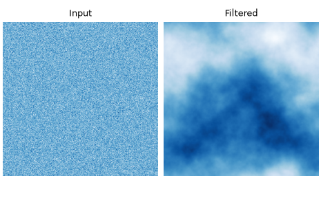
Here’s a simple FFT-based lowpass filter applied to an image of white noise.

This code will generate an image of white noise, use rfft2 to transform it to the frequency domain, apply a lowpass filter, and then transform back to the spatial domain with irfft2.

>>> import numpy as np
>>> import matplotlib.pyplot as plt
>>> from scipy.fft import rfft2, irfft2, fftfreq, rfftfreq
...
>>> rng = np.random.default_rng()
>>> m = 280  # Image size is m x m.

Generate an image of white noise:

>>> im = rng.normal(size=(m, m))

Transform to the frequency domain:

>>> f = rfft2(im)

Create a scaling filter that is applied in the frequency domain. This will be a lowpass filter:

>>> xfreqs, yfreqs = np.meshgrid(rfftfreq(m), fftfreq(m))
>>> r = np.hypot(xfreqs, yfreqs)
>>> r = r / r.max()
>>> r[0, 0] = 1

The power of r determines the “clumpiness” of the result:

>>> p = 2
>>> filt = r**-p

Apply the filter to f:

>>> f2 = filt * f

Convert back to the spatial domain with irfft2:

>>> im2 = irfft2(f2)

Take a look at the result:

>>> fig, (ax1, ax2) = plt.subplots(1, 2, constrained_layout=True)
>>> ax1.imshow(im, cmap='Blues')
>>> ax1.set_title('Input')
>>> ax1.set_axis_off()
>>> ax2.imshow(im2, cmap='Blues')
>>> ax2.set_title('Filtered')
>>> ax2.set_axis_off()
>>> plt.show()