1 # This example describe how to integrate ODEs with scipy.integrate module, and how
   2 # to use the matplotlib module to plot trajectories, direction fields and other
   3 # useful information.
   4 # 
   5 # == Presentation of the Lokta-Volterra Model ==
   6 # 
   7 # We will have a look at the Lokta-Volterra model, also known as the
   8 # predator-prey equations, which are a pair of first order, non-linear, differential
   9 # equations frequently used to describe the dynamics of biological systems in
  10 # which two species interact, one a predator and one its prey. They were proposed
  11 # independently by Alfred J. Lotka in 1925 and Vito Volterra in 1926:
  12 # du/dt =  a*u -   b*u*v
  13 # dv/dt = -c*v + d*b*u*v 
  14 # 
  15 # with the following notations:
  16 # 
  17 # *  u: number of preys (for example, rabbits)
  18 # 
  19 # *  v: number of predators (for example, foxes)  
  20 #   
  21 # * a, b, c, d are constant parameters defining the behavior of the population:    
  22 # 
  23 #   + a is the natural growing rate of rabbits, when there's no fox
  24 # 
  25 #   + b is the natural dying rate of rabbits, due to predation
  26 # 
  27 #   + c is the natural dying rate of fox, when there's no rabbit
  28 # 
  29 #   + d is the factor describing how many caught rabbits let create a new fox
  30 # 
  31 # We will use X=[u, v] to describe the state of both populations.
  32 # 
  33 # Definition of the equations:
  34 # 
  35 from numpy import *
  36 import pylab as p
  37 
  38 # Definition of parameters 
  39 a = 1.
  40 b = 0.1
  41 c = 1.5
  42 d = 0.75
  43 
  44 def dX_dt(X, t=0):
  45     """ Return the growth rate of fox and rabbit populations. """
  46     return array([ a*X[0] -   b*X[0]*X[1] ,  
  47                   -c*X[1] + d*b*X[0]*X[1] ])
  48 # 
  49 # === Population equilibrium ===
  50 # 
  51 # Before using !SciPy to integrate this system, we will have a closer look on 
  52 # position equilibrium. Equilibrium occurs when the growth rate is equal to 0.
  53 # This gives two fixed points:
  54 # 
  55 X_f0 = array([     0. ,  0.])
  56 X_f1 = array([ c/(d*b), a/b])
  57 all(dX_dt(X_f0) == zeros(2) ) and all(dX_dt(X_f1) == zeros(2)) # => True 
  58 # 
  59 # === Stability of the fixed points ===
  60 # Near theses two points, the system can be linearized:
  61 # dX_dt = A_f*X where A is the Jacobian matrix evaluated at the corresponding point.
  62 # We have to define the Jacobian matrix:
  63 # 
  64 def d2X_dt2(X, t=0):
  65     """ Return the Jacobian matrix evaluated in X. """
  66     return array([[a -b*X[1],   -b*X[0]     ],
  67                   [b*d*X[1] ,   -c +b*d*X[0]] ])  
  68 # 
  69 # So, near X_f0, which represents the extinction of both species, we have:
  70 # A_f0 = d2X_dt2(X_f0)                    # >>> array([[ 1. , -0. ],
  71 #                                         #            [ 0. , -1.5]])
  72 # 
  73 # Near X_f0, the number of rabbits increase and the population of foxes decrease.
  74 # The origin is a [http://en.wikipedia.org/wiki/Saddle_point saddle point].
  75 # 
  76 # Near X_f1, we have:
  77 A_f1 = d2X_dt2(X_f1)                    # >>> array([[ 0.  , -2.  ],
  78                                         #            [ 0.75,  0.  ]])
  79 
  80 # whose eigenvalues are +/- sqrt(c*a).j:
  81 lambda1, lambda2 = linalg.eigvals(A_f1) # >>> (1.22474j, -1.22474j)
  82 
  83 # They are imaginary number, so the fox and rabbit populations are periodic and
  84 # their period is given by:
  85 T_f1 = 2*pi/abs(lambda1)                # >>> 5.130199
  86 #         
  87 # == Integrating the ODE using scipy.integate ==
  88 # 
  89 # Now we will use the scipy.integrate module to integrate the ODEs.
  90 # This module offers a method named odeint, very easy to use to integrate ODEs:
  91 # 
  92 from scipy import integrate
  93 
  94 t = linspace(0, 15,  1000)              # time
  95 X0 = array([10, 5])                     # initials conditions: 10 rabbits and 5 foxes  
  96 
  97 X, infodict = integrate.odeint(dX_dt, X0, t, full_output=True)
  98 infodict['message']                     # >>> 'Integration successful.'
  99 # 
 100 # `infodict` is optional, and you can omit the `full_output` argument if you don't want it.
 101 # Type "info(odeint)" if you want more information about odeint inputs and outputs.
 102 # 
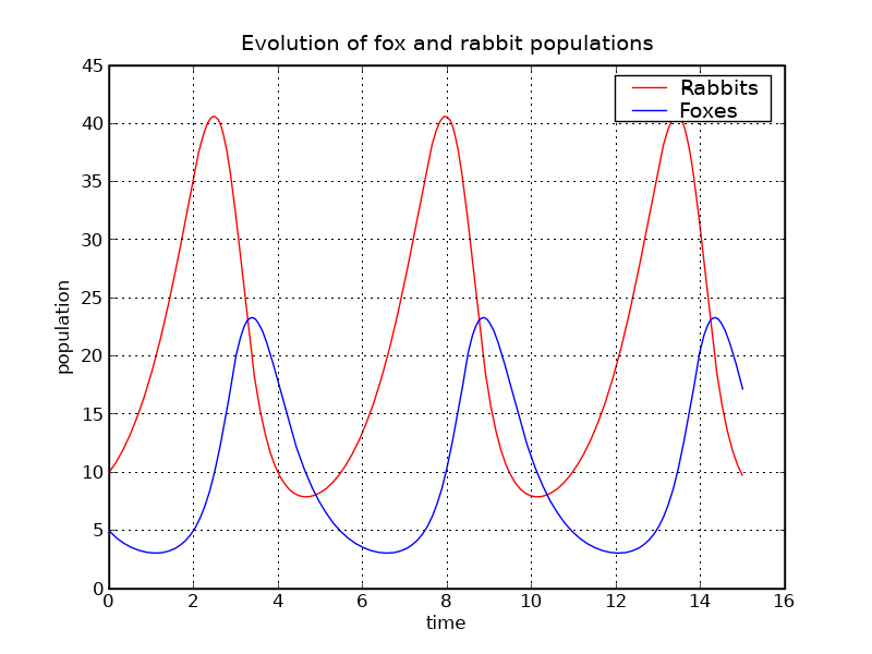
 103 # We can now use Matplotlib to plot the evolution of both populations:
 104 # 
 105 rabbits, foxes = X.T
 106 
 107 f1 = p.figure()
 108 p.plot(t, rabbits, 'r-', label='Rabbits')
 109 p.plot(t, foxes  , 'b-', label='Foxes')
 110 p.grid()
 111 p.legend(loc='best')
 112 p.xlabel('time')
 113 p.ylabel('population')
 114 p.title('Evolution of fox and rabbit populations')
 115 f1.savefig('rabbits_and_foxes_1.png')
 116 # 
 117 # 
 118 # The populations are indeed periodic, and their period is near to the T_f1 we calculated.
 119 # 
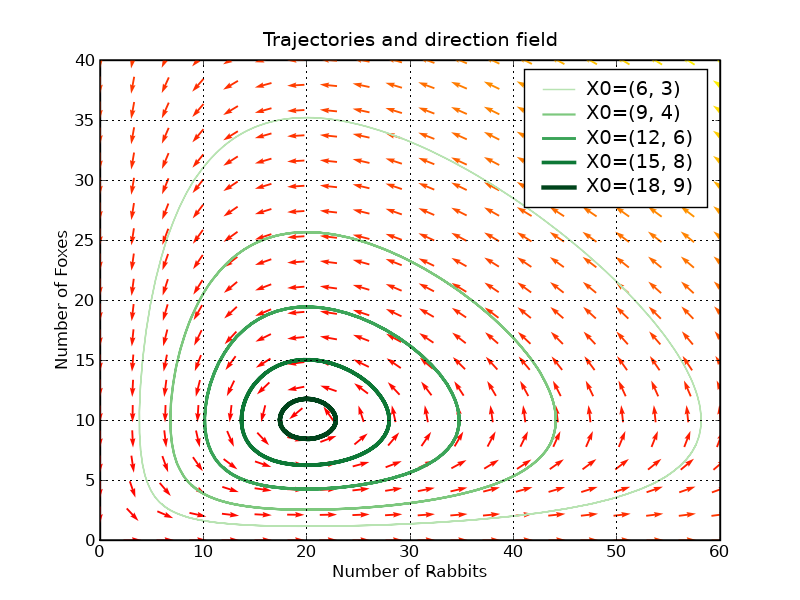
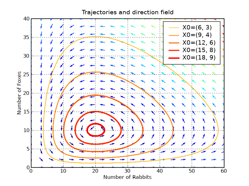
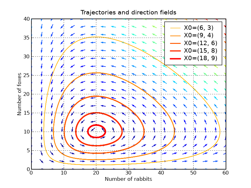
 120 # == Plotting direction fields and trajectories in the phase plane ==
 121 # 
 122 # We will plot some trajectories in a phase plane for different starting
 123 # points between X__f0 and X_f1.
 124 # 
 125 # We will use matplotlib's colormap to define colors for the trajectories.
 126 # These colormaps are very useful to make nice plots.
 127 # Have a look at [http://www.scipy.org/Cookbook/Matplotlib/Show_colormaps ShowColormaps] if you want more information.
 128 # 
 129 values  = linspace(0.3, 0.9, 5)                          # position of X0 between X_f0 and X_f1
 130 vcolors = p.cm.autumn_r(linspace(0.3, 1., len(values)))  # colors for each trajectory
 131 
 132 f2 = p.figure()
 133 
 134 #-------------------------------------------------------
 135 # plot trajectories
 136 for v, col in zip(values, vcolors): 
 137     X0 = v * X_f1                               # starting point
 138     X = integrate.odeint( dX_dt, X0, t)         # we don't need infodict here
 139     p.plot( X[:,0], X[:,1], lw=3.5*v, color=col, label='X0=(%.f, %.f)' % ( X0[0], X0[1]) )
 140 
 141 #-------------------------------------------------------
 142 # define a grid and compute direction at each point
 143 ymax = p.ylim(ymin=0)[1]                        # get axis limits
 144 xmax = p.xlim(xmin=0)[1] 
 145 nb_points   = 20                      
 146 
 147 x = linspace(0, xmax, nb_points)
 148 y = linspace(0, ymax, nb_points)
 149 
 150 X1 , Y1  = meshgrid(x, y)                       # create a grid
 151 DX1, DY1 = dX_dt([X1, Y1])                      # compute growth rate on the gridt
 152 M = (hypot(DX1, DY1))                           # Norm of the growth rate 
 153 M[ M == 0] = 1.                                 # Avoid zero division errors 
 154 DX1 /= M                                        # Normalize each arrows
 155 DY1 /= M                                  
 156 
 157 #-------------------------------------------------------
 158 # Drow direction fields, using matplotlib 's quiver function
 159 # I choose to plot normalized arrows and to use colors to give information on
 160 # the growth speed
 161 p.title('Trajectories and direction fields')
 162 Q = p.quiver(X1, Y1, DX1, DY1, M, pivot='mid', cmap=p.cm.jet)
 163 p.xlabel('Number of rabbits')
 164 p.ylabel('Number of foxes')
 165 p.legend()
 166 p.grid()
 167 p.xlim(0, xmax)
 168 p.ylim(0, ymax)
 169 f2.savefig('rabbits_and_foxes_2.png')
 170 # 
 171 # 
 172 # We can see on this graph that an intervention on fox or rabbit populations can
 173 # have non intuitive effects. If, in order to decrease the number of rabbits,
 174 # we introduce foxes, this can lead to an increase of rabbits in the long run,
 175 # if that intervention happens at a bad moment.
 176 # 
 177 # 
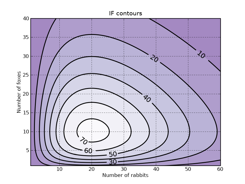
 178 # == Plotting contours ==
 179 # 
 180 # We can verify that the function IF defined below remains constant along a trajectory:
 181 # 
 182 def IF(X):
 183     u, v = X
 184     return u**(c/a) * v * exp( -(b/a)*(d*u+v) )
 185 
 186 # We will verify that IF remains constant for different trajectories
 187 for v in values: 
 188     X0 = v * X_f1                               # starting point
 189     X = integrate.odeint( dX_dt, X0, t)         
 190     I = IF(X.T)                                 # compute IF along the trajectory
 191     I_mean = I.mean()
 192     delta = 100 * (I.max()-I.min())/I_mean
 193     print 'X0=(%2.f,%2.f) => I ~ %.1f |delta = %.3G %%' % (X0[0], X0[1], I_mean, delta)
 194 
 195 # >>> X0=( 6, 3) => I ~ 20.8 |delta = 6.19E-05 %
 196 #     X0=( 9, 4) => I ~ 39.4 |delta = 2.67E-05 %
 197 #     X0=(12, 6) => I ~ 55.7 |delta = 1.82E-05 %
 198 #     X0=(15, 8) => I ~ 66.8 |delta = 1.12E-05 %
 199 #     X0=(18, 9) => I ~ 72.4 |delta = 4.68E-06 %
 200 # 
 201 # Potting iso-contours of IF can be a good representation of trajectories,
 202 # without having to integrate the ODE
 203 # 
 204 #-------------------------------------------------------
 205 # plot iso contours
 206 nb_points = 80                              # grid size 
 207 
 208 x = linspace(0, xmax, nb_points)    
 209 y = linspace(0, ymax, nb_points)
 210 
 211 X2 , Y2  = meshgrid(x, y)                   # create the grid
 212 Z2 = IF([X2, Y2])                           # compute IF on each point
 213 
 214 f3 = p.figure()
 215 CS = p.contourf(X2, Y2, Z2, cmap=p.cm.Purples_r, alpha=0.5)
 216 CS2 = p.contour(X2, Y2, Z2, colors='black', linewidths=2. )
 217 p.clabel(CS2, inline=1, fontsize=16, fmt='%.f')
 218 p.grid()
 219 p.xlabel('Number of rabbits')
 220 p.ylabel('Number of foxes')
 221 p.ylim(1, ymax)
 222 p.xlim(1, xmax)
 223 p.title('IF contours')
 224 f3.savefig('rabbits_and_foxes_3.png')
 225 p.show()
 226 # 
 227 # 
 228 # # vim: set et sts=4 sw=4: