1 #! /usr/bin/env python
   2 # -*- coding: utf-8 -*-
   3 
   4 """
   5 http://www.scipy.org/Cookbook/Least_Squares_Circle
   6 """
   7 
   8 from numpy import *
   9 
  10 # Coordinates of the 2D points
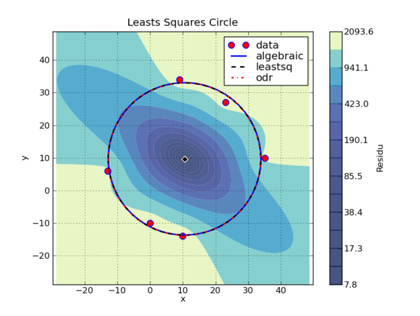
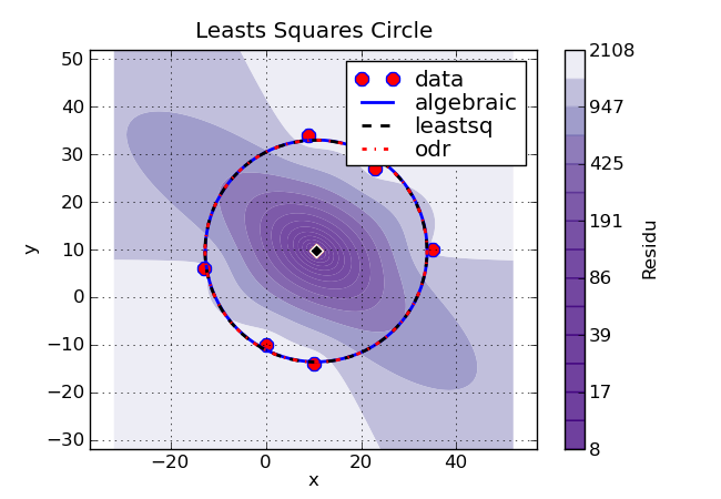
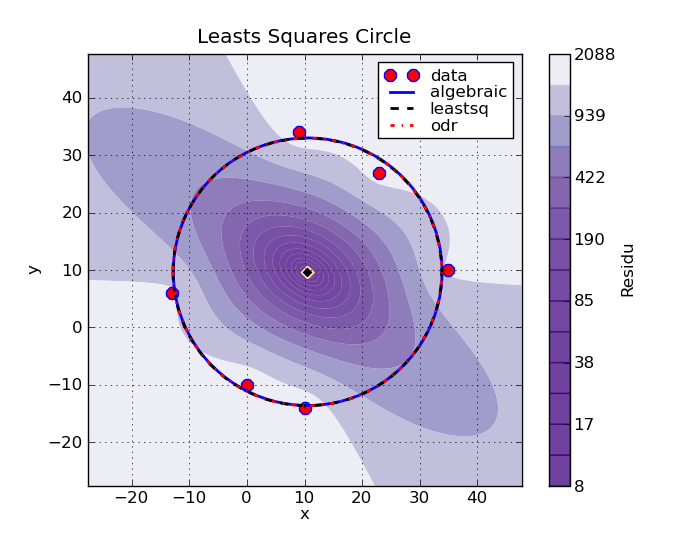
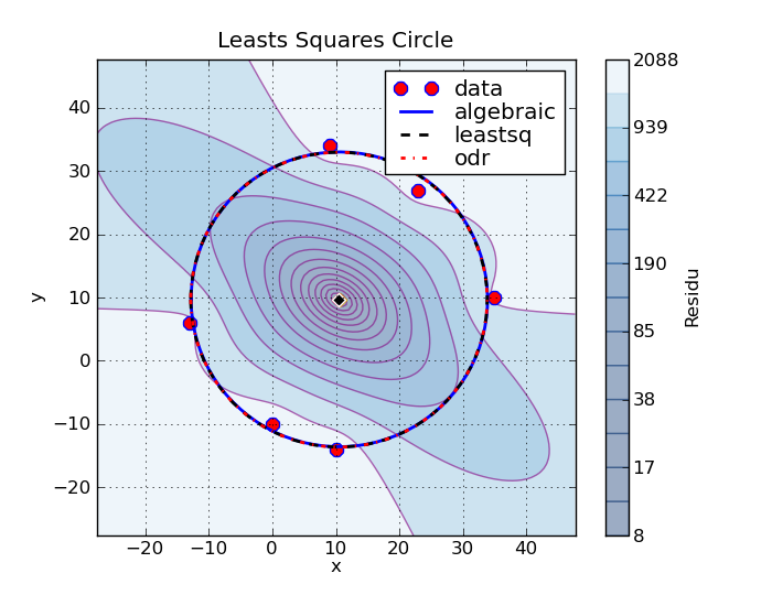
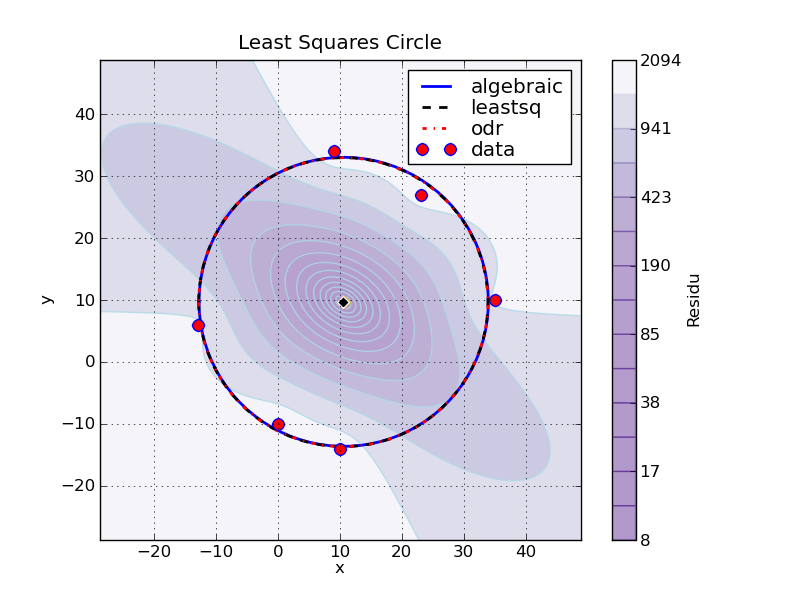
  11 x = r_[  9,  35, -13,  10,  23,   0]
  12 y = r_[ 34,  10,   6, -14,  27, -10]
  13 
  14 # == METHOD 1 ==
  15 method_1 = 'algebraic'
  16 
  17 # coordinates of the barycenter
  18 x_m = mean(x)
  19 y_m = mean(y)
  20 
  21 # calculation of the reduced coordinates
  22 u = x - x_m
  23 v = y - y_m
  24 
  25 # linear system defining the center in reduced coordinates (uc, vc):
  26 #    Suu * uc +  Suv * vc = (Suuu + Suvv)/2
  27 #    Suv * uc +  Svv * vc = (Suuv + Svvv)/2
  28 
  29 Suv  = sum(u*v)
  30 Suu  = sum(u**2)
  31 Svv  = sum(v**2)
  32 Suuv = sum(u**2 * v)
  33 Suvv = sum(u * v**2)
  34 Suuu = sum(u**3)
  35 Svvv = sum(v**3)
  36 
  37 # Solving the linear system
  38 A = array([ [ Suu, Suv ], [Suv, Svv]])
  39 B = array([ Suuu + Suvv, Svvv + Suuv ])/2.0
  40 uc, vc = linalg.solve(A, B)
  41 
  42 xc_1 = x_m + uc
  43 yc_1 = y_m + vc
  44 
  45 # Calculation of all distances from the center (xc_1, yc_1)
  46 Ri_1     = sqrt((x-xc_1)**2 + (y-yc_1)**2)
  47 R_1      = mean(Ri_1)
  48 residu_1 = sum((Ri_1-R_1)**2)
  49 
  50 #  == METHOD 2 ==
  51 from scipy      import optimize
  52 
  53 method_2 = "leastsq"
  54 
  55 def calc_R(c):
  56     """ calculate the distance of each 2D points from the center c=(xc, yc) """
  57     return sqrt((x-c[0])**2 + (y-c[1])**2)
  58 
  59 def calc_ecart(c):
  60     """ calculate the algebraic distance between the 2D points and the mean circle centered at c=(xc, yc) """
  61     Ri = calc_R(c)
  62     return Ri - Ri.mean()
  63 
  64 center_estimate = x_m, y_m
  65 center_2, ier = optimize.leastsq(calc_ecart, center_estimate)
  66 
  67 xc_2, yc_2 = center_2
  68 Ri_2       = calc_R(center_2)
  69 R_2        = Ri_2.mean()
  70 residu_2   = sum((Ri_2 - R_2)**2)
  71 
  72 # == METHOD 3 ==
  73 from scipy      import  odr
  74 
  75 method_3 = "odr"
  76 
  77 def calc_f(beta, x):
  78     """ implicit function of the circle """
  79     xc, yc, r = beta
  80     return (x[0]-xc)**2 + (x[1]-yc)**2 -r**2
  81 
  82 def calc_estimate(data):
  83     """ Return a first estimation on the parameter from the data  """
  84     xc0, yc0 = data.x.mean(axis=1)
  85     r0 = sqrt((data.x[0]-xc0)**2 +(data.x[1] -yc0)**2).mean()
  86     return xc0, yc0, r0
  87 
  88 # for implicit function :
  89 #       data.x contains both coordinates of the points
  90 #       data.y is the dimensionality of the response
  91 lsc_data  = odr.Data(row_stack([x, y]), y=1)
  92 lsc_model = odr.Model(calc_f, implicit=True, estimate=calc_estimate)
  93 lsc_odr   = odr.ODR(lsc_data, lsc_model)
  94 lsc_out   = lsc_odr.run()
  95 
  96 xc_3, yc_3, R_3 = lsc_out.beta
  97 Ri_3 = calc_R([xc_3, yc_3])
  98 residu_3 = sum((Ri_3 - R_3)**2)
  99 
 100 # Summary
 101 fmt = '%-15s %10.5f %10.5f %10.5f %10.6f %10.6f'
 102 print '\n%-15s %10s %10s %10s %10s %10s' % tuple('METHOD Xc Yc Rc std(Ri) residu'.split())
 103 print '-'*(15 +5*(10+1))
 104 print  fmt % (method_1, xc_1, yc_1, R_1, Ri_1.std(), residu_1)
 105 print  fmt % (method_2, xc_2, yc_2, R_2, Ri_2.std(), residu_2)
 106 print  fmt % (method_3, xc_3, yc_3, R_3, Ri_3.std(), residu_3)
 107 
 108 # plotting functions
 109 
 110 from matplotlib import pyplot as p, cm
 111 
 112 f = p.figure()
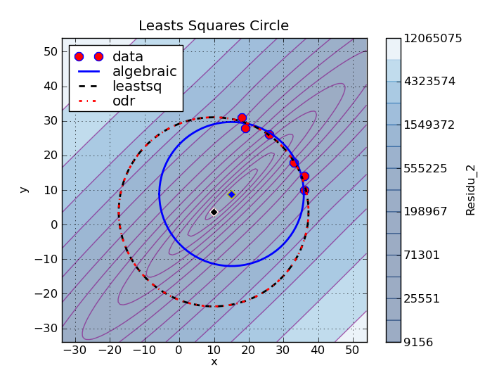
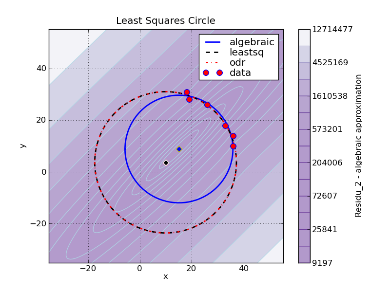
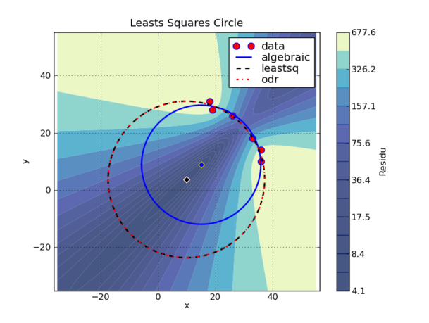
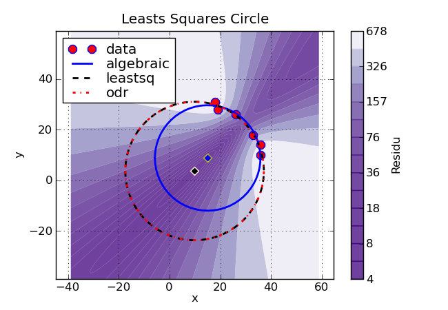
 113 p.plot(x, y, 'ro', label='data', ms=9, mec='b', mew=1)
 114 
 115 theta_fit = linspace(-pi, pi, 180)
 116 
 117 x_fit1 = xc_1 + R_1*cos(theta_fit)
 118 y_fit1 = yc_1 + R_1*sin(theta_fit)
 119 p.plot(x_fit1, y_fit1, 'b-' , label=method_1, lw=2)
 120 
 121 x_fit2 = xc_2 + R_2*cos(theta_fit)
 122 y_fit2 = yc_2 + R_2*sin(theta_fit)
 123 p.plot(x_fit2, y_fit2, 'k--', label=method_2, lw=2)
 124 
 125 x_fit3 = xc_3 + R_3*cos(theta_fit)
 126 y_fit3 = yc_3 + R_3*sin(theta_fit)
 127 p.plot(x_fit3, y_fit3, 'r-.', label=method_3, lw=2)
 128 
 129 p.plot([xc_1], [yc_1], 'bD', mec='y', mew=1)
 130 p.plot([xc_2], [yc_2], 'gD', mec='r', mew=1)
 131 p.plot([xc_3], [yc_3], 'kD', mec='w', mew=1)
 132 
 133 # draw
 134 p.axis('equal')
 135 p.xlabel('x')
 136 p.ylabel('y')
 137 p.legend(loc='best',labelspacing=0.1)
 138 
 139 # plot the residu fields
 140 nb_pts = 100
 141 
 142 p.draw()
 143 xmin, xmax = p.xlim()
 144 ymin, ymax = p.ylim()
 145 
 146 vmin = min(xmin, ymin)
 147 vmax = max(xmax, ymax)
 148 
 149 xg, yg = ogrid[vmin:vmax:nb_pts*1j, vmin:vmax:nb_pts*1j]
 150 xg = xg[..., newaxis]
 151 yg = yg[..., newaxis]
 152 
 153 Rig    = sqrt( (xg - x)**2 + (yg - y)**2 )
 154 Rig_m  = Rig.mean(axis=2)[..., newaxis]
 155 residu = sum( (Rig-Rig_m)**2 ,axis=2)
 156 
 157 lvl = exp(linspace(log(residu.min()), log(residu.max()), 15))
 158 
 159 p.contourf(xg.flat, yg.flat, residu.T, lvl, alpha=0.75, cmap=cm.YlGnBu_r)
 160 cbar = p.colorbar(format='%.1f')
 161 cbar.set_label('Residu')
 162 p.xlim(xmin=vmin, xmax=vmax)
 163 p.ylim(ymin=vmin, ymax=vmax)
 164 
 165 p.grid()
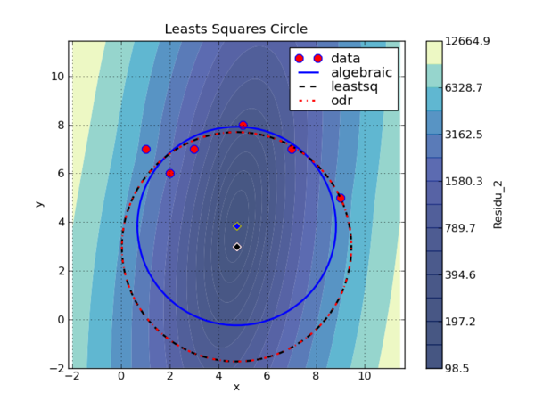
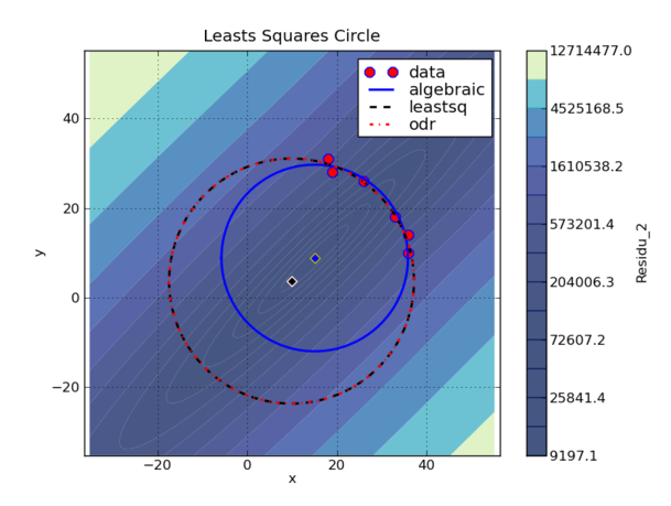
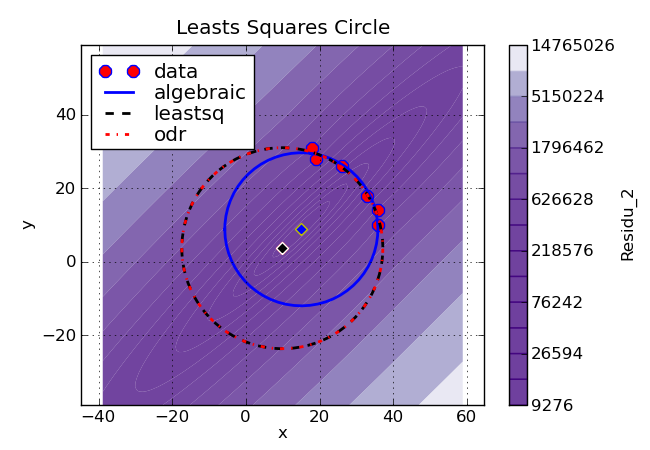
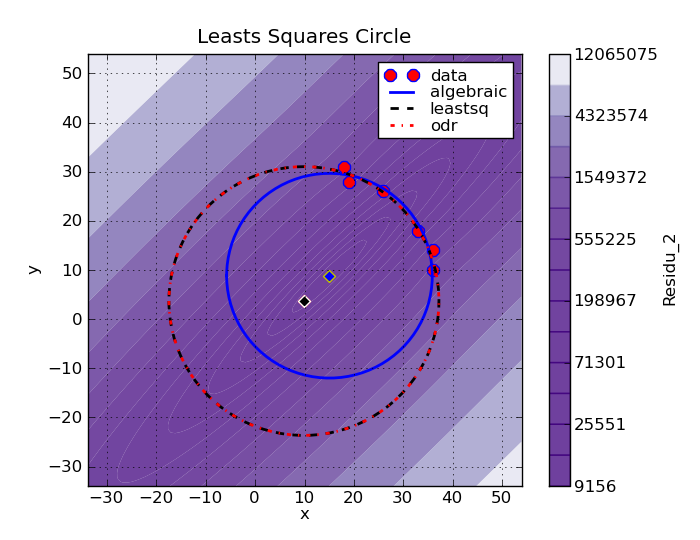
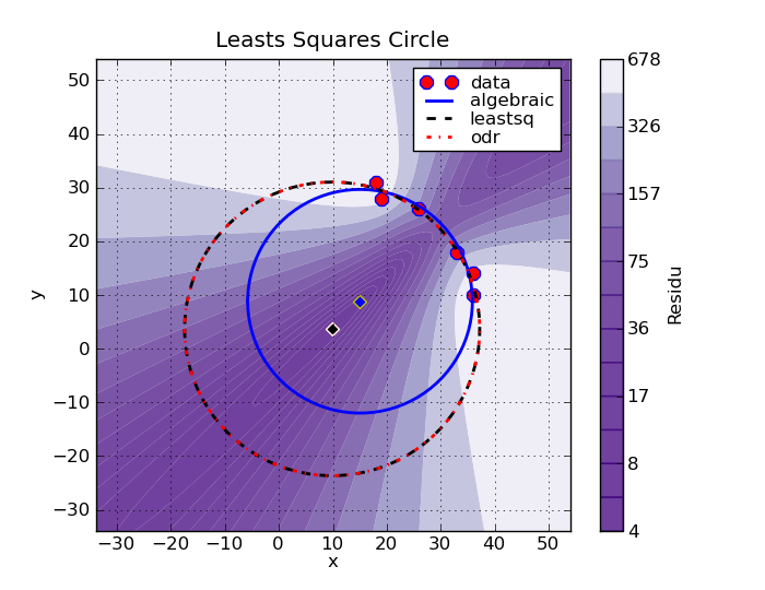
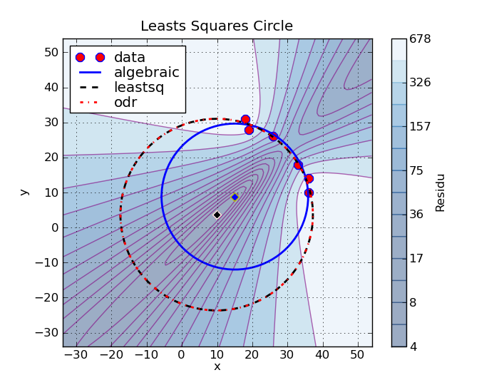
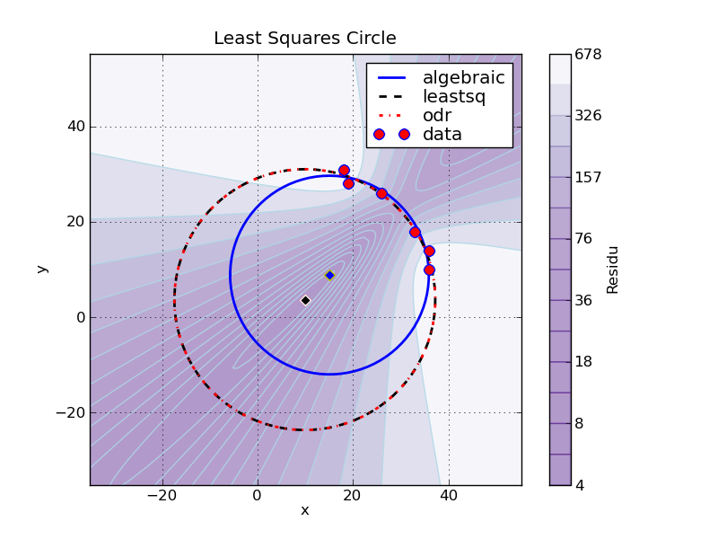
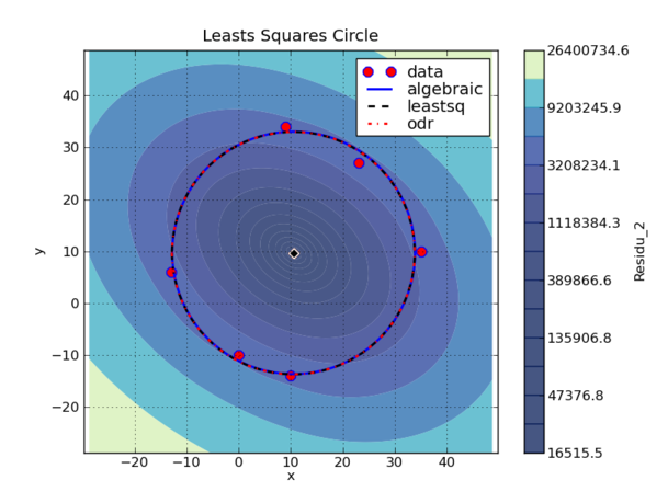
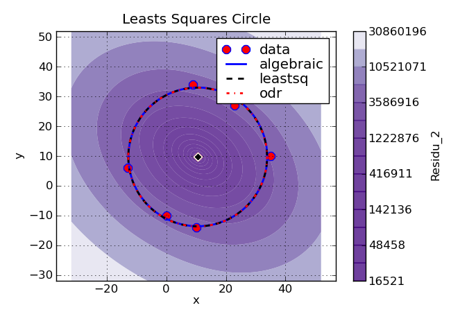
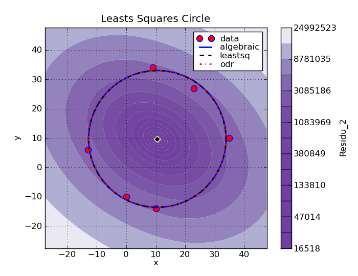
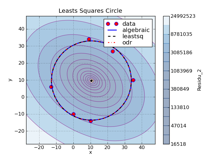
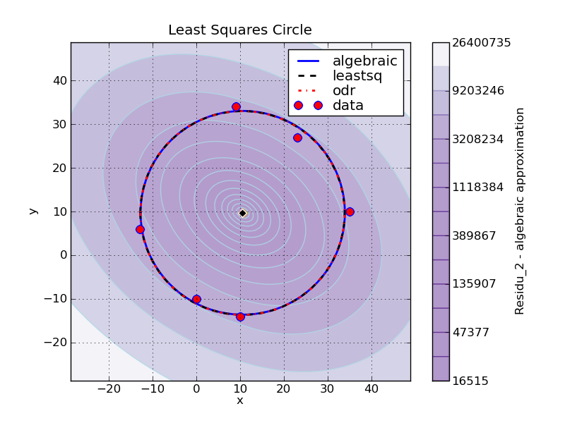
 166 p.title('Leasts Squares Circle')
 167 p.show()
 168 # vim: set et sts=4 sw=4: