Polynomial interpolation based INVersion of CDF (PINV)

• Required: PDF

• Optional: CDF, mode, center

• Speed:

  • Set-up: (very) slow

  • Sampling: (very) fast

Polynomial interpolation based INVersion of CDF (PINV) is an inversion method that only requires the density function to sample from a distribution. It is based on Polynomial interpolation of the PPF and Gauss-Lobatto integration of the PDF. It provides control over the interpolation error and integration error. Its primary purpose is to provide very fast sampling which is nearly the same for any given distribution at the cost of moderate to slow setup time. It is the fastest known inversion method for the fixed-parameter case.

The inversion method is the simplest and most flexible to sample nonuniform random variates. For a target distribution with CDF \(F\) and a uniform random variate \(U\) sampled from \(\text{Uniform}(0, 1)\), a random variate X is generated by transforming the uniform random variate \(U\) using the PPF (inverse CDF) of the distribution:

\[X = F^{-1}(U)\]

This method is suitable for stochastic simulations because of its advantages. Some of the most attractive are:

• It preserves the structural properties of the uniform random number sampler.

• Transforms a uniform random variate \(U\) one-to-one into non-uniform random variates \(X\).

• Easy and efficient sampling from truncated distributions.

Unfortunately, the PPF is rarely available in closed form or too slow when available. For many distributions, the CDF is also not easy to obtain. This method addresses both the shortcomings. The user only has to provide the PDF and optionally a point near the mode (called “center”) together with the size of the maximal acceptable error. It uses a combination of an adaptive and a simple Gauss-Lobatto quadrature to obtain the CDF and Newton’s interpolation to obtain the PPF. The method is not exact, as it only produces random variates of the approximated distribution. Nevertheless, the maximal tolerated approximation error can be set close to the machine precision. The concept of u-error is used to measure and control the error. It is defined as:

\[\epsilon_{u}(u) = | u - F\left(F^{-1}_{a}(u)\right) |\]

where \(u \in (0, 1)\) is a quantile where we want to measure the error and \(F^{-1}_a\) is the approximated PPF of the given distribution.

The maximal u-error is the criterion for approximation errors when calculating the CDF and PPF numerically. The maximal tolerated u-error of an algorithm is called the u-resolution of the algorithm and denoted by \(\epsilon_{u}\):

\[\sup_{u \in (0,1)} | u - F\left(F^{-1}_{a}(u)\right) | \le \epsilon_{u}\]

The main advantage of the u-error is that it can be easily computed if the CDF is available. We refer to [1] for a more detailed discussion.

Also, the method only works for bounded distributions. In case of infinite tails, the ends of the tails are cut off such that the area under them is less than or equal to \(0.05\epsilon_{u}\).

There are some restrictions for the given distribution:

• The support of the distribution (i.e., the region where the PDF is strictly positive) must be connected. In practice this means, that the region where PDF is “not too small” must be connected. Unimodal densities satisfy this condition. If this condition is violated then the domain of the distribution might be truncated.

• When the PDF is integrated numerically, then the given PDF must be continuous and should be smooth.

• The PDF must be bounded.

• The algorithm has problems when the distribution has heavy tails (as then the inverse CDF becomes very steep at 0 or 1) and the requested u-resolution is very small. E.g., the Cauchy distribution is likely to show this problem when the requested u-resolution is less than 1.e-12.

Following four steps are carried out by the algorithm during setup:

• Computing the end points of the distribution: If a finite support is given, this step is skipped. Otherwise, the ends of the tails are cut off such that the area under them is less than or equal to \(0.05\epsilon_{u}\).

• The domain is divided into subintervals to compute the CDF and PPF.

• The CDF is computed using Gauss-Lobatto quadrature such that the integration error is at most \(0.05I_{0}\epsilon_{u}\) where \(I_{0}\) is approximately the total area under the PDF.

• The PPF is computed using Newton’s interpolating formula with maximum interpolation error \(0.9\epsilon_{u}\).

To initialize the generator to sample from a standard normal distribution, do:

>>> import numpy as np
>>> from scipy.stats.sampling import NumericalInversePolynomial
>>> class StandardNormal:
...     def pdf(self, x):
...         return np.exp(-0.5 * x*x)
...
>>> dist = StandardNormal()
>>> urng = np.random.default_rng()
>>> rng = NumericalInversePolynomial(dist, random_state=urng)

The generator has been setup and we can start sampling from our distribution:

>>> rng.rvs((5, 3))
array([[-1.52449963,  1.31933688,  2.05884468],
       [ 0.48883931,  0.15207903, -0.02150773],
       [ 1.11486463,  1.95449597, -0.30724928],
       [ 0.9854643 ,  0.29867424,  0.7560304 ],
       [-0.61776203,  0.16033378, -1.00933003]])

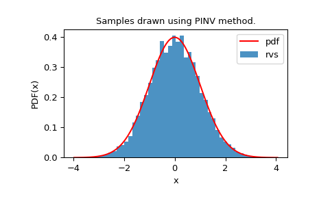
We can look at the histogram of the random variates to check how well they fit our distribution:

>>> import matplotlib.pyplot as plt
>>> from scipy.stats import norm
>>> from scipy.stats.sampling import NumericalInversePolynomial
>>> class StandardNormal:
...     def pdf(self, x):
...         return np.exp(-0.5 * x*x)
...
>>> dist = StandardNormal()
>>> urng = np.random.default_rng()
>>> rng = NumericalInversePolynomial(dist, random_state=urng)
>>> rvs = rng.rvs(10000)
>>> x = np.linspace(rvs.min()-0.1, rvs.max()+0.1, num=10000)
>>> fx = norm.pdf(x)
>>> plt.plot(x, fx, "r-", label="pdf")
>>> plt.hist(rvs, bins=50, density=True, alpha=0.8, label="rvs")
>>> plt.xlabel("x")
>>> plt.ylabel("PDF(x)")
>>> plt.title("Samples drawn using PINV method.")
>>> plt.legend()
>>> plt.show()

The maximum tolerated error (i.e. u-resolution) can be changed by passing the u_resolution keyword during initialization:

>>> rng = NumericalInversePolynomial(dist, u_resolution=1e-12,
...                                  random_state=urng)

This leads to a more accurate approximation of the PPF and the generated RVs follow the exact distribution more closely. Although, note that it comes at the cost of an expensive setup.

The setup time mainly depends on the number of times the PDF is evaluated. It is more costly for PDFs that are difficult to evaluate. Note that we can ignore the normalization constant to speed up the evaluations of the PDF. PDF evaluations increase during setup for small values of u_resolution.

>>> from scipy.stats.sampling import NumericalInversePolynomial
>>> class StandardNormal:
...     def __init__(self):
...         self.callbacks = 0
...     def pdf(self, x):
...         self.callbacks += 1
...         return np.exp(-0.5 * x*x)
...
>>> dist = StandardNormal()
>>> urng = np.random.default_rng()
>>> # u_resolution = 10^-8
>>> # => less PDF evaluations required
>>> # => faster setup
>>> rng = NumericalInversePolynomial(dist, u_resolution=1e-8,
...                                  random_state=urng)
>>> dist.callbacks
4095        # may vary
>>> dist.callbacks = 0  # reset the number of callbacks
>>> # u_resolution = 10^-10 (default)
>>> # => more PDF evaluations required
>>> # => slow setup
>>> rng = NumericalInversePolynomial(dist, u_resolution=1e-10,
...                                  random_state=urng)
>>> dist.callbacks
11454       # may vary
>>> dist.callbacks = 0  # reset the number of callbacks
>>> # u_resolution = 10^-12
>>> # => lots of PDF evaluations required
>>> # => very slow setup
>>> rng = NumericalInversePolynomial(dist, u_resolution=1e-12,
...                                  random_state=urng)
13902     # may vary

As we can see, the number of PDF evaluations required is very high and a fast PDF is critical to the algorithm. Though, this helps reduce the number of subintervals required to achieve the error goal which saves memory and makes sampling fast. NumericalInverseHermite is a similar inversion method that inverts the CDF based on Hermite interpolation and provides control over the maximum tolerated error via u-resolution. But it makes use of a lot more intervals compared to NumericalInversePolynomial:

>>> from scipy.stats.sampling import NumericalInverseHermite
>>> # NumericalInverseHermite accepts a `tol` parameter to set the
>>> # u-resolution of the generator.
>>> rng_hermite = NumericalInverseHermite(norm(), tol=1e-12)
>>> rng_hermite.intervals
3000
>>> rng_poly = NumericalInversePolynomial(norm(), u_resolution=1e-12)
>>> rng_poly.intervals
252

When exact CDF of a distribution is available, one can estimate the u-error achieved by the algorithm by calling the u_error method:

>>> from scipy.special import ndtr
>>> class StandardNormal:
...     def pdf(self, x):
...         return np.exp(-0.5 * x*x)
...     def cdf(self, x):
...         return ndtr(x)
...
>>> dist = StandardNormal()
>>> urng = np.random.default_rng()
>>> rng = NumericalInversePolynomial(dist, random_state=urng)
>>> rng.u_error(sample_size=100_000)
UError(max_error=8.785949745515609e-11, mean_absolute_error=2.9307548109436816e-11)

u_error runs a monte carlo simulation with a given number of samples to estimate the u-error. In the above example, 100,000 samples are used by the simulation to approximate the u-error. It returns the maximum u-error (max_error) and the mean absolute u-error (mean_absolute_error) in a UError namedtuple. As we can see, max_error is below the default u_resolution (1e-10).

It is also possible to evaluate the PPF of the given distribution once the generator is initialized:

>>> rng.ppf(0.975)
1.959963985701268
>>> norm.ppf(0.975)
1.959963984540054

We can use this, for example, to check the maximum and mean absolute u-error:

>>> u = np.linspace(0.001, 0.999, num=1_000_000)
>>> u_errors = np.abs(u - dist.cdf(rng.ppf(u)))
>>> u_errors.max()
8.78600525666684e-11
>>> u_errors.mean()
2.9321444940323206e-11

The approximate PPF method provided by the generator is much faster to evaluate than the exact PPF of the distribution.

During setup, a table of CDF points is stored that can be used to approximate the CDF once the generator has been created:

>>> rng.cdf(1.959963984540054)
0.9750000000042454
>>> norm.cdf(1.959963984540054)
0.975

We can use this to check if the integration error while computing the CDF exceeds \(0.05I_{0}\epsilon_{u}\). Here \(I_0\) is \(\sqrt{2\pi}\) (the normalization constant for the standard normal distribution):

>>> x = np.linspace(-10, 10, num=100_000)
>>> x_error = np.abs(dist.cdf(x) - rng.cdf(x))
>>> x_error.max()
4.506062190046123e-12
>>> I0 = np.sqrt(2*np.pi)
>>> max_integration_error = 0.05 * I0 * 1e-10
>>> x_error.max() <= max_integration_error
True

The CDF table computed during setup is used to evaluate the CDF and only some further fine-tuning is required. This reduces the calls to the PDF but as the fine-tuning step uses the simple Gauss-Lobatto quadrature, the PDF is called several times, slowing down the computation.

References

[1]

Derflinger, Gerhard, Wolfgang Hörmann, and Josef Leydold. “Random variate generation by numerical inversion when only the density is known.” ACM Transactions on Modeling and Computer Simulation (TOMACS) 20.4 (2010): 1-25.