Probability distributions#

There are two general distribution classes that have been implemented for encapsulating continuous random variables and discrete random variables. Over 80 continuous random variables (RVs) and 10 discrete random variables have been implemented using these classes. For mathematical reference information about individual distributions, please see Continuous Statistical Distributions and Discrete Statistical Distributions.

All of the statistics functions are located in the sub-package scipy.stats and a fairly complete listing of these functions and random variables available can also be obtained from the docstring for the stats sub-package.

In the discussion below, we mostly focus on continuous RVs. Nearly everything also applies to discrete variables, but we point out some differences here: Specific points for discrete distributions.

In the code samples below, we assume that the scipy.stats package is imported as

>>> from scipy import stats

and in some cases we assume that individual objects are imported as

>>> from scipy.stats import norm

All distributions

Getting help#

First of all, all distributions are accompanied with help functions. To obtain just some basic information, we print the relevant docstring: print(stats.norm.__doc__).

To find the support, i.e., upper and lower bounds of the distribution, call:

>>> print('bounds of distribution lower: %s, upper: %s' % norm.support())
bounds of distribution lower: -inf, upper: inf

We can list all methods and properties of the distribution with dir(norm). As it turns out, some of the methods are private, although they are not named as such (their names do not start with a leading underscore), for example veccdf, are only available for internal calculation (those methods will give warnings when one tries to use them, and will be removed at some point).

To obtain the real main methods, we list the methods of the frozen distribution. (We explain the meaning of a frozen distribution below).

>>> rv = norm()
>>> dir(rv)  # reformatted
['__class__', '__delattr__', '__dict__', '__dir__', '__doc__', '__eq__',
 '__format__', '__ge__', '__getattribute__', '__gt__', '__hash__',
 '__init__', '__le__', '__lt__', '__module__', '__ne__', '__new__',
 '__reduce__', '__reduce_ex__', '__repr__', '__setattr__', '__sizeof__',
 '__str__', '__subclasshook__', '__weakref__', 'a', 'args', 'b', 'cdf',
 'dist', 'entropy', 'expect', 'interval', 'isf', 'kwds', 'logcdf',
 'logpdf', 'logpmf', 'logsf', 'mean', 'median', 'moment', 'pdf', 'pmf',
 'ppf', 'random_state', 'rvs', 'sf', 'stats', 'std', 'var']

Finally, we can obtain the list of available distribution through introspection:

>>> dist_continu = [d for d in dir(stats) if
...                 isinstance(getattr(stats, d), stats.rv_continuous)]
>>> dist_discrete = [d for d in dir(stats) if
...                  isinstance(getattr(stats, d), stats.rv_discrete)]
>>> print('number of continuous distributions: %d' % len(dist_continu))
number of continuous distributions: 108
>>> print('number of discrete distributions:   %d' % len(dist_discrete))
number of discrete distributions:   20

Common methods#

The main public methods for continuous RVs are:

rvs: Random Variates
pdf: Probability Density Function
cdf: Cumulative Distribution Function
sf: Survival Function (1-CDF)
ppf: Percent Point Function (Inverse of CDF)
isf: Inverse Survival Function (Inverse of SF)
stats: Return mean, variance, (Fisher’s) skew, or (Fisher’s) kurtosis
moment: non-central moments of the distribution

Let’s take a normal RV as an example.

>>> norm.cdf(0)
0.5

To compute the cdf at a number of points, we can pass a list or a numpy array.

>>> norm.cdf([-1., 0, 1])
array([ 0.15865525,  0.5,  0.84134475])
>>> import numpy as np
>>> norm.cdf(np.array([-1., 0, 1]))
array([ 0.15865525,  0.5,  0.84134475])

Thus, the basic methods, such as pdf, cdf, and so on, are vectorized.

Other generally useful methods are supported too:

>>> norm.mean(), norm.std(), norm.var()
(0.0, 1.0, 1.0)
>>> norm.stats(moments="mv")
(array(0.0), array(1.0))

To find the median of a distribution, we can use the percent point function ppf, which is the inverse of the cdf:

>>> norm.ppf(0.5)
0.0

To generate a sequence of random variates, use the size keyword argument:

>>> norm.rvs(size=3)
array([-0.35687759,  1.34347647, -0.11710531])   # random

Don’t think that norm.rvs(5) generates 5 variates:

>>> norm.rvs(5)
5.471435163732493  # random

Here, 5 with no keyword is being interpreted as the first possible keyword argument, loc, which is the first of a pair of keyword arguments taken by all continuous distributions. This brings us to the topic of the next subsection.

Random number generation#

Drawing random numbers relies on generators from numpy.random package. In the examples above, the specific stream of random numbers is not reproducible across runs. To achieve reproducibility, you can explicitly seed a random number generator. In NumPy, a generator is an instance of numpy.random.Generator. Here is the canonical way to create a generator:

>>> from numpy.random import default_rng
>>> rng = default_rng()

And fixing the seed can be done like this:

>>> # do NOT copy this value
>>> rng = default_rng(301439351238479871608357552876690613766)

Warning

Do not use this number or common values such as 0. Using just a small set of seeds to instantiate larger state spaces means that there are some initial states that are impossible to reach. This creates some biases if everyone uses such values. A good way to get a seed is to use a numpy.random.SeedSequence:

>>> from numpy.random import SeedSequence
>>> print(SeedSequence().entropy)
301439351238479871608357552876690613766  # random

The random_state parameter in distributions accepts an instance of numpy.random.Generator class, or an integer, which is then used to seed an internal Generator object:

>>> norm.rvs(size=5, random_state=rng)
array([ 0.47143516, -1.19097569,  1.43270697, -0.3126519 , -0.72058873])  # random

For further info, see NumPy’s documentation.

To learn more about the random number samplers implemented in SciPy, see non-uniform random number sampling tutorial and quasi monte carlo tutorial

Shifting and scaling#

All continuous distributions take loc and scale as keyword parameters to adjust the location and scale of the distribution, e.g., for the standard normal distribution, the location is the mean and the scale is the standard deviation.

>>> norm.stats(loc=3, scale=4, moments="mv")
(array(3.0), array(16.0))

In many cases, the standardized distribution for a random variable X is obtained through the transformation (X - loc) / scale. The default values are loc = 0 and scale = 1.

Smart use of loc and scale can help modify the standard distributions in many ways. To illustrate the scaling further, the cdf of an exponentially distributed RV with mean \(1/\lambda\) is given by

\[F(x) = 1 - \exp(-\lambda x)\]

By applying the scaling rule above, it can be seen that by taking scale = 1./lambda we get the proper scale.

>>> from scipy.stats import expon
>>> expon.mean(scale=3.)
3.0

Note

Distributions that take shape parameters may require more than simple application of loc and/or scale to achieve the desired form. For example, the distribution of 2-D vector lengths given a constant vector of length \(R\) perturbed by independent N(0, \(\sigma^2\)) deviations in each component is rice(\(R/\sigma\), scale= \(\sigma\)). The first argument is a shape parameter that needs to be scaled along with \(x\).

The uniform distribution is also interesting:

>>> from scipy.stats import uniform
>>> uniform.cdf([0, 1, 2, 3, 4, 5], loc=1, scale=4)
array([ 0.  ,  0.  ,  0.25,  0.5 ,  0.75,  1.  ])

Finally, recall from the previous paragraph that we are left with the problem of the meaning of norm.rvs(5). As it turns out, calling a distribution like this, the first argument, i.e., the 5, gets passed to set the loc parameter. Let’s see:

>>> np.mean(norm.rvs(5, size=500))
5.0098355106969992  # random

Thus, to explain the output of the example of the last section: norm.rvs(5) generates a single normally distributed random variate with mean loc=5, because of the default size=1.

We recommend that you set loc and scale parameters explicitly, by passing the values as keywords rather than as arguments. Repetition can be minimized when calling more than one method of a given RV by using the technique of Freezing a Distribution, as explained below.

Shape parameters#

While a general continuous random variable can be shifted and scaled with the loc and scale parameters, some distributions require additional shape parameters. For instance, the gamma distribution with density

\[\gamma(x, a) = \frac{\lambda (\lambda x)^{a-1}}{\Gamma(a)} e^{-\lambda x}\;,\]

requires the shape parameter \(a\). Observe that setting \(\lambda\) can be obtained by setting the scale keyword to \(1/\lambda\).

Let’s check the number and name of the shape parameters of the gamma distribution. (We know from the above that this should be 1.)

>>> from scipy.stats import gamma
>>> gamma.numargs
1
>>> gamma.shapes
'a'

Now, we set the value of the shape variable to 1 to obtain the exponential distribution, so that we compare easily whether we get the results we expect.

>>> gamma(1, scale=2.).stats(moments="mv")
(array(2.0), array(4.0))

Notice that we can also specify shape parameters as keywords:

>>> gamma(a=1, scale=2.).stats(moments="mv")
(array(2.0), array(4.0))

Freezing a distribution#

Passing the loc and scale keywords time and again can become quite bothersome. The concept of freezing a RV is used to solve such problems.

>>> rv = gamma(1, scale=2.)

By using rv we no longer have to include the scale or the shape parameters anymore. Thus, distributions can be used in one of two ways, either by passing all distribution parameters to each method call (such as we did earlier) or by freezing the parameters for the instance of the distribution. Let us check this:

>>> rv.mean(), rv.std()
(2.0, 2.0)

This is, indeed, what we should get.

Broadcasting#

The basic methods pdf, and so on, satisfy the usual numpy broadcasting rules. For example, we can calculate the critical values for the upper tail of the t distribution for different probabilities and degrees of freedom.

>>> stats.t.isf([0.1, 0.05, 0.01], [[10], [11]])
array([[ 1.37218364,  1.81246112,  2.76376946],
       [ 1.36343032,  1.79588482,  2.71807918]])

Here, the first row contains the critical values for 10 degrees of freedom and the second row for 11 degrees of freedom (d.o.f.). Thus, the broadcasting rules give the same result of calling isf twice:

>>> stats.t.isf([0.1, 0.05, 0.01], 10)
array([ 1.37218364,  1.81246112,  2.76376946])
>>> stats.t.isf([0.1, 0.05, 0.01], 11)
array([ 1.36343032,  1.79588482,  2.71807918])

If the array with probabilities, i.e., [0.1, 0.05, 0.01] and the array of degrees of freedom i.e., [10, 11, 12], have the same array shape, then element-wise matching is used. As an example, we can obtain the 10% tail for 10 d.o.f., the 5% tail for 11 d.o.f. and the 1% tail for 12 d.o.f. by calling

>>> stats.t.isf([0.1, 0.05, 0.01], [10, 11, 12])
array([ 1.37218364,  1.79588482,  2.68099799])

Specific points for discrete distributions#

Discrete distributions have mostly the same basic methods as the continuous distributions. However pdf is replaced by the probability mass function pmf, no estimation methods, such as fit, are available, and scale is not a valid keyword parameter. The location parameter, keyword loc, can still be used to shift the distribution.

The computation of the cdf requires some extra attention. In the case of continuous distribution, the cumulative distribution function is, in most standard cases, strictly monotonic increasing in the bounds (a,b) and has, therefore, a unique inverse. The cdf of a discrete distribution, however, is a step function, hence the inverse cdf, i.e., the percent point function, requires a different definition:

ppf(q) = min{x : cdf(x) >= q, x integer}

For further info, see the docs here.

We can look at the hypergeometric distribution as an example

>>> from scipy.stats import hypergeom
>>> [M, n, N] = [20, 7, 12]

If we use the cdf at some integer points and then evaluate the ppf at those cdf values, we get the initial integers back, for example

>>> x = np.arange(4) * 2
>>> x
array([0, 2, 4, 6])
>>> prb = hypergeom.cdf(x, M, n, N)
>>> prb
array([  1.03199174e-04,   5.21155831e-02,   6.08359133e-01,
         9.89783282e-01])
>>> hypergeom.ppf(prb, M, n, N)
array([ 0.,  2.,  4.,  6.])

If we use values that are not at the kinks of the cdf step function, we get the next higher integer back:

>>> hypergeom.ppf(prb + 1e-8, M, n, N)
array([ 1.,  3.,  5.,  7.])
>>> hypergeom.ppf(prb - 1e-8, M, n, N)
array([ 0.,  2.,  4.,  6.])

Fitting distributions#

The main additional methods of the not frozen distribution are related to the estimation of distribution parameters:

fit: maximum likelihood estimation of distribution parameters, including location
and scale
fit_loc_scale: estimation of location and scale when shape parameters are given
nnlf: negative log likelihood function
expect: calculate the expectation of a function against the pdf or pmf

Performance issues and cautionary remarks#

The performance of the individual methods, in terms of speed, varies widely by distribution and method. The results of a method are obtained in one of two ways: either by explicit calculation, or by a generic algorithm that is independent of the specific distribution.

Explicit calculation, on the one hand, requires that the method is directly specified for the given distribution, either through analytic formulas or through special functions in scipy.special or numpy.random for rvs. These are usually relatively fast calculations.

The generic methods, on the other hand, are used if the distribution does not specify any explicit calculation. To define a distribution, only one of pdf or cdf is necessary; all other methods can be derived using numeric integration and root finding. However, these indirect methods can be very slow. As an example, rgh = stats.gausshyper.rvs(0.5, 2, 2, 2, size=100) creates random variables in a very indirect way and takes about 19 seconds for 100 random variables on my computer, while one million random variables from the standard normal or from the t distribution take just above one second.

Remaining issues#

The distributions in scipy.stats have recently been corrected and improved and gained a considerable test suite; however, a few issues remain:

The distributions have been tested over some range of parameters; however, in some corner ranges, a few incorrect results may remain.
The maximum likelihood estimation in fit does not work with default starting parameters for all distributions and the user needs to supply good starting parameters. Also, for some distribution using a maximum likelihood estimator might inherently not be the best choice.

Building specific distributions#

The next examples shows how to build your own distributions. Further examples show the usage of the distributions and some statistical tests.

Making a continuous distribution, i.e., subclassing `rv_continuous`#

Making continuous distributions is fairly simple.

>>> from scipy import stats
>>> class deterministic_gen(stats.rv_continuous):
...     def _cdf(self, x):
...         return np.where(x < 0, 0., 1.)
...     def _stats(self):
...         return 0., 0., 0., 0.

>>> deterministic = deterministic_gen(name="deterministic")
>>> deterministic.cdf(np.arange(-3, 3, 0.5))
array([ 0.,  0.,  0.,  0.,  0.,  0.,  1.,  1.,  1.,  1.,  1.,  1.])

Interestingly, the pdf is now computed automatically:

>>> deterministic.pdf(np.arange(-3, 3, 0.5))
array([  0.00000000e+00,   0.00000000e+00,   0.00000000e+00,
         0.00000000e+00,   0.00000000e+00,   0.00000000e+00,
         5.83333333e+04,   4.16333634e-12,   4.16333634e-12,
         4.16333634e-12,   4.16333634e-12,   4.16333634e-12])

Be aware of the performance issues mentioned in Performance issues and cautionary remarks. The computation of unspecified common methods can become very slow, since only general methods are called, which, by their very nature, cannot use any specific information about the distribution. Thus, as a cautionary example:

>>> from scipy.integrate import quad
>>> quad(deterministic.pdf, -1e-1, 1e-1)
(4.163336342344337e-13, 0.0)

But this is not correct: the integral over this pdf should be 1. Let’s make the integration interval smaller:

>>> quad(deterministic.pdf, -1e-3, 1e-3)  # warning removed
(1.000076872229173, 0.0010625571718182458)

This looks better. However, the problem originated from the fact that the pdf is not specified in the class definition of the deterministic distribution.

Subclassing `rv_discrete`#

In the following, we use stats.rv_discrete to generate a discrete distribution that has the probabilities of the truncated normal for the intervals centered around the integers.

General info

From the docstring of rv_discrete, help(stats.rv_discrete),

“You can construct an arbitrary discrete rv where P{X=xk} = pk by passing to the rv_discrete initialization method (through the values= keyword) a tuple of sequences (xk, pk) which describes only those values of X (xk) that occur with nonzero probability (pk).”

Next to this, there are some further requirements for this approach to work:

The keyword name is required.
The support points of the distribution xk have to be integers.
The number of significant digits (decimals) needs to be specified.

In fact, if the last two requirements are not satisfied, an exception may be raised or the resulting numbers may be incorrect.

An example

Let’s do the work. First:

>>> npoints = 20   # number of integer support points of the distribution minus 1
>>> npointsh = npoints // 2
>>> npointsf = float(npoints)
>>> nbound = 4   # bounds for the truncated normal
>>> normbound = (1+1/npointsf) * nbound   # actual bounds of truncated normal
>>> grid = np.arange(-npointsh, npointsh+2, 1)   # integer grid
>>> gridlimitsnorm = (grid-0.5) / npointsh * nbound   # bin limits for the truncnorm
>>> gridlimits = grid - 0.5   # used later in the analysis
>>> grid = grid[:-1]
>>> probs = np.diff(stats.truncnorm.cdf(gridlimitsnorm, -normbound, normbound))
>>> gridint = grid

And, finally, we can subclass rv_discrete:

>>> normdiscrete = stats.rv_discrete(values=(gridint,
...              np.round(probs, decimals=7)), name='normdiscrete')

Now that we have defined the distribution, we have access to all common methods of discrete distributions.

>>> print('mean = %6.4f, variance = %6.4f, skew = %6.4f, kurtosis = %6.4f' %
...       normdiscrete.stats(moments='mvsk'))
mean = -0.0000, variance = 6.3302, skew = 0.0000, kurtosis = -0.0076

>>> nd_std = np.sqrt(normdiscrete.stats(moments='v'))

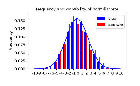
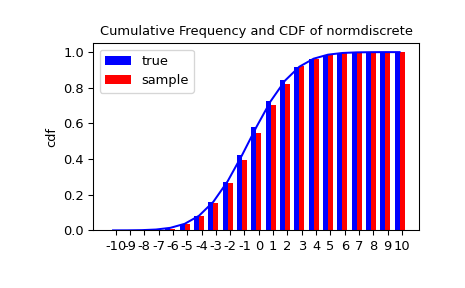
Testing the implementation

Let’s generate a random sample and compare observed frequencies with the probabilities.

>>> n_sample = 500
>>> rvs = normdiscrete.rvs(size=n_sample)
>>> f, l = np.histogram(rvs, bins=gridlimits)
>>> sfreq = np.vstack([gridint, f, probs*n_sample]).T
>>> print(sfreq)
[[-1.00000000e+01  0.00000000e+00  2.95019349e-02]  # random
 [-9.00000000e+00  0.00000000e+00  1.32294142e-01]
 [-8.00000000e+00  0.00000000e+00  5.06497902e-01]
 [-7.00000000e+00  2.00000000e+00  1.65568919e+00]
 [-6.00000000e+00  1.00000000e+00  4.62125309e+00]
 [-5.00000000e+00  9.00000000e+00  1.10137298e+01]
 [-4.00000000e+00  2.60000000e+01  2.24137683e+01]
 [-3.00000000e+00  3.70000000e+01  3.89503370e+01]
 [-2.00000000e+00  5.10000000e+01  5.78004747e+01]
 [-1.00000000e+00  7.10000000e+01  7.32455414e+01]
 [ 0.00000000e+00  7.40000000e+01  7.92618251e+01]
 [ 1.00000000e+00  8.90000000e+01  7.32455414e+01]
 [ 2.00000000e+00  5.50000000e+01  5.78004747e+01]
 [ 3.00000000e+00  5.00000000e+01  3.89503370e+01]
 [ 4.00000000e+00  1.70000000e+01  2.24137683e+01]
 [ 5.00000000e+00  1.10000000e+01  1.10137298e+01]
 [ 6.00000000e+00  4.00000000e+00  4.62125309e+00]
 [ 7.00000000e+00  3.00000000e+00  1.65568919e+00]
 [ 8.00000000e+00  0.00000000e+00  5.06497902e-01]
 [ 9.00000000e+00  0.00000000e+00  1.32294142e-01]
 [ 1.00000000e+01  0.00000000e+00  2.95019349e-02]]

"An X-Y histogram plot showing the distribution of random variates. A blue trace shows a normal bell curve. A blue bar chart perfectly approximates the curve showing the true distribution. A red bar chart representing the sample is well described by the blue trace but not exact."

"An X-Y histogram plot showing the cumulative distribution of random variates. A blue trace shows a CDF for a typical normal distribution. A blue bar chart perfectly approximates the curve showing the true distribution. A red bar chart representing the sample is well described by the blue trace but not exact."

Next, we can test whether our sample was generated by our norm-discrete distribution. This also verifies whether the random numbers were generated correctly.

The chisquare test requires that there are a minimum number of observations in each bin. We combine the tail bins into larger bins so that they contain enough observations.

>>> f2 = np.hstack([f[:5].sum(), f[5:-5], f[-5:].sum()])
>>> p2 = np.hstack([probs[:5].sum(), probs[5:-5], probs[-5:].sum()])
>>> ch2, pval = stats.chisquare(f2, p2*n_sample)

>>> print('chisquare for normdiscrete: chi2 = %6.3f pvalue = %6.4f' % (ch2, pval))
chisquare for normdiscrete: chi2 = 12.466 pvalue = 0.4090  # random

The pvalue in this case is high, so we can be quite confident that our random sample was actually generated by the distribution.