Spearman correlation coefficient#
The Spearman rank-order correlation coefficient is a nonparametric measure of the monotonicity of the relationship between two datasets.
Consider the following data from [1], which studied the relationship between free proline (an amino acid) and total collagen (a protein often found in connective tissue) in unhealthy human livers.
The x and y arrays below record measurements of the two compounds. The
observations are paired: each free proline measurement was taken from the same
liver as the total collagen measurement at the same index.
import numpy as np
# total collagen (mg/g dry weight of liver)
x = np.array([7.1, 7.1, 7.2, 8.3, 9.4, 10.5, 11.4])
# free proline (μ mole/g dry weight of liver)
y = np.array([2.8, 2.9, 2.8, 2.6, 3.5, 4.6, 5.0])
These data were analyzed in [2] using Spearman’s correlation coefficient, a
statistic sensitive to monotonic correlation between the samples, implemented
as scipy.stats.spearmanr.
from scipy import stats
res = stats.spearmanr(x, y)
res.statistic
np.float64(0.7000000000000001)
The value of this statistic tends to be high (close to 1) for samples with a strongly positive ordinal correlation, low (close to -1) for samples with a strongly negative ordinal correlation, and small in magnitude (close to zero) for samples with weak ordinal correlation.
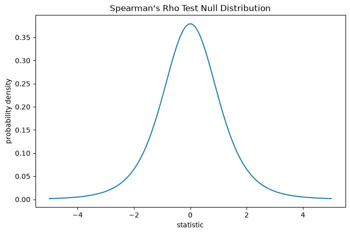
The test is performed by comparing the observed value of the statistic against the null distribution: the distribution of statistic values derived under the null hypothesis that total collagen and free proline measurements are independent.
For this test, the statistic can be transformed such that the null distribution
for large samples is Student’s t distribution with len(x) - 2 degrees of freedom.
import matplotlib.pyplot as plt
dof = len(x)-2  # len(x) == len(y)
dist = stats.t(df=dof)
t_vals = np.linspace(-5, 5, 100)
pdf = dist.pdf(t_vals)
fig, ax = plt.subplots(figsize=(8, 5))

def plot(ax):  # we'll reuse this
    ax.plot(t_vals, pdf)
    ax.set_title("Spearman's Rho Test Null Distribution")
    ax.set_xlabel("statistic")
    ax.set_ylabel("probability density")

plot(ax)
plt.show()
The comparison is quantified by the p-value: the proportion of values in the null distribution as extreme or more extreme than the observed value of the statistic. In a two-sided test in which the statistic is positive, elements of the null distribution greater than the transformed statistic and elements of the null distribution less than the negative of the observed statistic are both considered “more extreme”.
fig, ax = plt.subplots(figsize=(8, 5))
plot(ax)
rs = res.statistic  # original statistic
transformed = rs * np.sqrt(dof / ((rs+1.0)*(1.0-rs)))
pvalue = dist.cdf(-transformed) + dist.sf(transformed)
annotation = (f'p-value={pvalue:.4f}\n(shaded area)')
props = dict(facecolor='black', width=1, headwidth=5, headlength=8)
_ = ax.annotate(annotation, (2.7, 0.025), (3, 0.03), arrowprops=props)
i = t_vals >= transformed
ax.fill_between(t_vals[i], y1=0, y2=pdf[i], color='C0')
i = t_vals <= -transformed
ax.fill_between(t_vals[i], y1=0, y2=pdf[i], color='C0')
ax.set_xlim(-5, 5)
ax.set_ylim(0, 0.1)
plt.show()
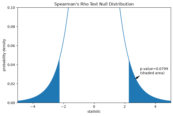
res.pvalue
np.float64(0.07991669030889918)
If the p-value is “small” - that is, if there is a low probability of sampling data from independent distributions that produces such an extreme value of the statistic - this may be taken as evidence against the null hypothesis in favor of the alternative: the distribution of total collagen and free proline are not independent. Note that:
The inverse is not true; that is, the test is not used to provide evidence for the null hypothesis.
The threshold for values that will be considered “small” is a choice that should be made before the data is analyzed [3] with consideration of the risks of both false positives (incorrectly rejecting the null hypothesis) and false negatives (failure to reject a false null hypothesis).
Small p-values are not evidence for a large effect; rather, they can only provide evidence for a “significant” effect, meaning that they are unlikely to have occurred under the null hypothesis.
Suppose that before performing the experiment, the authors had reason to predict a positive correlation between the total collagen and free proline measurements, and that they had chosen to assess the plausibility of the null hypothesis against a one-sided alternative: free proline has a positive ordinal correlation with total collagen. In this case, only those values in the null distribution that are as great or greater than the observed statistic are considered to be more extreme.
res = stats.spearmanr(x, y, alternative='greater')
res.statistic
np.float64(0.7000000000000001)
fig, ax = plt.subplots(figsize=(8, 5))
plot(ax)
pvalue = dist.sf(transformed)
annotation = (f'p-value={pvalue:.6f}\n(shaded area)')
props = dict(facecolor='black', width=1, headwidth=5, headlength=8)
_ = ax.annotate(annotation, (3, 0.018), (3.5, 0.03), arrowprops=props)
i = t_vals >= transformed
ax.fill_between(t_vals[i], y1=0, y2=pdf[i], color='C0')
ax.set_xlim(1, 5)
ax.set_ylim(0, 0.1)
plt.show()
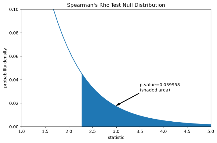
res.pvalue
np.float64(0.03995834515444959)
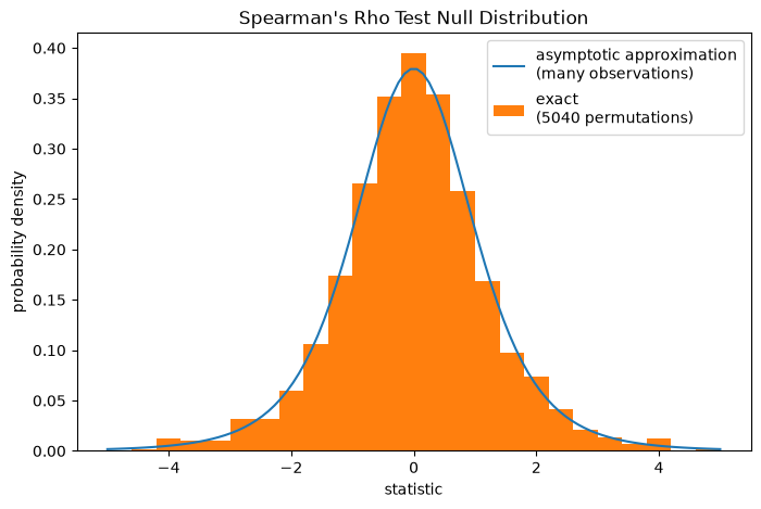
Note that the t-distribution provides an asymptotic approximation of the null
distribution; it is only accurate for samples with many observations. For small
samples, it may be more appropriate to perform a permutation test [4]: Under the
null hypothesis that total collagen and free proline are independent, each of
the free proline measurements were equally likely to have been observed with any
of the total collagen measurements. Therefore, we can form an exact null
distribution by calculating the statistic under each possible pairing of
elements between x and y.
def statistic(x):  # explore all possible pairings by permuting `x`
    rs = stats.spearmanr(x, y).statistic  # ignore pvalue
    transformed = rs * np.sqrt(dof / ((rs+1.0)*(1.0-rs)))
    return transformed
ref = stats.permutation_test((x,), statistic, alternative='greater',
                             permutation_type='pairings')
fig, ax = plt.subplots(figsize=(8, 5))
plot(ax)
ax.hist(ref.null_distribution, np.linspace(-5, 5, 26),
        density=True)
ax.legend(['asymptotic approximation\n(many observations)',
           f'exact \n({len(ref.null_distribution)} permutations)'])
plt.show()
ref.pvalue
np.float64(0.04563492063492063)