scipy.stats.skellam#

scipy.stats.skellam = <scipy.stats._discrete_distns.skellam_gen object>[source]#

A Skellam discrete random variable.

As an instance of the rv_discrete class, skellam object inherits from it a collection of generic methods (see below for the full list), and completes them with details specific for this particular distribution.

Methods

rvs(mu1, mu2, loc=0, size=1, random_state=None)	Random variates.
pmf(k, mu1, mu2, loc=0)	Probability mass function.
logpmf(k, mu1, mu2, loc=0)	Log of the probability mass function.
cdf(k, mu1, mu2, loc=0)	Cumulative distribution function.
logcdf(k, mu1, mu2, loc=0)	Log of the cumulative distribution function.
sf(k, mu1, mu2, loc=0)	Survival function (also defined as `1 - cdf`, but sf is sometimes more accurate).
logsf(k, mu1, mu2, loc=0)	Log of the survival function.
ppf(q, mu1, mu2, loc=0)	Percent point function (inverse of `cdf` — percentiles).
isf(q, mu1, mu2, loc=0)	Inverse survival function (inverse of `sf`).
stats(mu1, mu2, loc=0, moments=’mv’)	Mean(‘m’), variance(‘v’), skew(‘s’), and/or kurtosis(‘k’).
entropy(mu1, mu2, loc=0)	(Differential) entropy of the RV.
expect(func, args=(mu1, mu2), loc=0, lb=None, ub=None, conditional=False)	Expected value of a function (of one argument) with respect to the distribution.
median(mu1, mu2, loc=0)	Median of the distribution.
mean(mu1, mu2, loc=0)	Mean of the distribution.
var(mu1, mu2, loc=0)	Variance of the distribution.
std(mu1, mu2, loc=0)	Standard deviation of the distribution.
interval(confidence, mu1, mu2, loc=0)	Confidence interval with equal areas around the median.

Notes

Probability distribution of the difference of two correlated or uncorrelated Poisson random variables.

Let $k_1$ and $k_2$ be two Poisson-distributed r.v. with expected values $\lambda_1$ and $\lambda_2$ . Then, $k_1 - k_2$ follows a Skellam distribution with parameters $\mu_1 = \lambda_1 - \rho \sqrt{\lambda_1 \lambda_2}$ and $\mu_2 = \lambda_2 - \rho \sqrt{\lambda_1 \lambda_2}$ , where $\rho$ is the correlation coefficient between $k_1$ and $k_2$ . If the two Poisson-distributed r.v. are independent then $\rho = 0$ .

Parameters $\mu_1$ and $\mu_2$ must be strictly positive.

For details see: https://en.wikipedia.org/wiki/Skellam_distribution

skellam takes $\mu_1$ and $\mu_2$ as shape parameters.

The probability mass function above is defined in the “standardized” form. To shift distribution use the loc parameter. Specifically, skellam.pmf(k, mu1, mu2, loc) is identically equivalent to skellam.pmf(k - loc, mu1, mu2).

Examples

>>> import numpy as np
>>> from scipy.stats import skellam
>>> import matplotlib.pyplot as plt
>>> fig, ax = plt.subplots(1, 1)

Get the support:

>>> mu1, mu2 = 15, 8
>>> lb, ub = skellam.support(mu1, mu2)

Calculate the first four moments:

>>> mean, var, skew, kurt = skellam.stats(mu1, mu2, moments='mvsk')

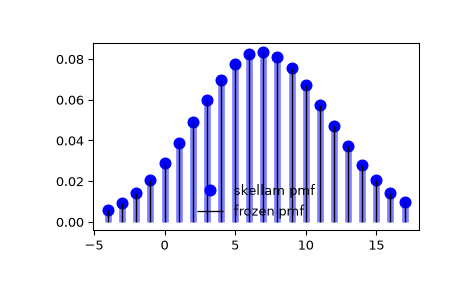
Display the probability mass function (pmf):

>>> x = np.arange(skellam.ppf(0.01, mu1, mu2),
...               skellam.ppf(0.99, mu1, mu2))
>>> ax.plot(x, skellam.pmf(x, mu1, mu2), 'bo', ms=8, label='skellam pmf')
>>> ax.vlines(x, 0, skellam.pmf(x, mu1, mu2), colors='b', lw=5, alpha=0.5)

Alternatively, the distribution object can be called (as a function) to fix the shape and location. This returns a “frozen” RV object holding the given parameters fixed.

Freeze the distribution and display the frozen pmf:

>>> rv = skellam(mu1, mu2)
>>> ax.vlines(x, 0, rv.pmf(x), colors='k', linestyles='-', lw=1,
...         label='frozen pmf')
>>> ax.legend(loc='best', frameon=False)
>>> plt.show()

../../_images/scipy-stats-skellam-1_00_00.png

Check accuracy of cdf and ppf:

>>> prob = skellam.cdf(x, mu1, mu2)
>>> np.allclose(x, skellam.ppf(prob, mu1, mu2))
True

Generate random numbers:

>>> r = skellam.rvs(mu1, mu2, size=1000)