scipy.stats.sampling.DiscreteGuideTable#

class scipy.stats.sampling.DiscreteGuideTable(dist, *, domain=None, guide_factor=1, random_state=None)#

Discrete Guide Table method.

The Discrete Guide Table method samples from arbitrary, but finite, probability vectors. It uses the probability vector of size \(N\) or a probability mass function with a finite support to generate random numbers from the distribution. Discrete Guide Table has a very slow set up (linear with the vector length) but provides very fast sampling.

Parameters:

distarray_like or object, optional

Probability vector (PV) of the distribution. If PV isn’t available, an instance of a class with a pmf method is expected. The signature of the PMF is expected to be: def pmf(self, k: int) -> float. i.e. it should accept a Python integer and return a Python float.

domainint, optional

Support of the PMF. If a probability vector (pv) is not available, a finite domain must be given. i.e. the PMF must have a finite support. Default is None. When None:

If a support method is provided by the distribution object dist, it is used to set the domain of the distribution.
Otherwise, the support is assumed to be (0, len(pv)). When this parameter is passed in combination with a probability vector, domain[0] is used to relocate the distribution from (0, len(pv)) to (domain[0], domain[0]+len(pv)) and domain[1] is ignored. See Notes and tutorial for a more detailed explanation.

guide_factor: int, optional

Size of the guide table relative to length of PV. Larger guide tables result in faster generation time but require a more expensive setup. Sizes larger than 3 are not recommended. If the relative size is set to 0, sequential search is used. Default is 1.

random_state{None, int, numpy.random.Generator,

numpy.random.RandomState}, optional

A NumPy random number generator or seed for the underlying NumPy random number generator used to generate the stream of uniform random numbers. If random_state is None (or np.random), the numpy.random.RandomState singleton is used. If random_state is an int, a new RandomState instance is used, seeded with random_state. If random_state is already a Generator or RandomState instance then that instance is used.

Notes

This method works when either a finite probability vector is available or the PMF of the distribution is available. In case a PMF is only available, the finite support (domain) of the PMF must also be given. It is recommended to first obtain the probability vector by evaluating the PMF at each point in the support and then using it instead.

DGT samples from arbitrary but finite probability vectors. Random numbers are generated by the inversion method, i.e.

Generate a random number U ~ U(0,1).
Find smallest integer I such that F(I) = P(X<=I) >= U.

Step (2) is the crucial step. Using sequential search requires O(E(X)) comparisons, where E(X) is the expectation of the distribution. Indexed search, however, uses a guide table to jump to some I’ <= I near I to find X in constant time. Indeed the expected number of comparisons is reduced to 2, when the guide table has the same size as the probability vector (this is the default). For larger guide tables this number becomes smaller (but is always larger than 1), for smaller tables it becomes larger. For the limit case of table size 1 the algorithm simply does sequential search.

On the other hand the setup time for guide table is O(N), where N denotes the length of the probability vector (for size 1 no preprocessing is required). Moreover, for very large guide tables memory effects might even reduce the speed of the algorithm. So we do not recommend to use guide tables that are more than three times larger than the given probability vector. If only a few random numbers have to be generated, (much) smaller table sizes are better. The size of the guide table relative to the length of the given probability vector can be set by the guide_factor parameter.

If a probability vector is given, it must be a 1-dimensional array of non-negative floats without any inf or nan values. Also, there must be at least one non-zero entry otherwise an exception is raised.

By default, the probability vector is indexed starting at 0. However, this can be changed by passing a domain parameter. When domain is given in combination with the PV, it has the effect of relocating the distribution from (0, len(pv)) to (domain[0], domain[0] + len(pv)). domain[1] is ignored in this case.

References

[1]

UNU.RAN reference manual, Section 5.8.4, “DGT - (Discrete) Guide Table method (indexed search)” https://statmath.wu.ac.at/unuran/doc/unuran.html#DGT

[2]

H.C. Chen and Y. Asau (1974). On generating random variates from an empirical distribution, AIIE Trans. 6, pp. 163-166.

Examples

>>> from scipy.stats.sampling import DiscreteGuideTable
>>> import numpy as np

To create a random number generator using a probability vector, use:

>>> pv = [0.1, 0.3, 0.6]
>>> urng = np.random.default_rng()
>>> rng = DiscreteGuideTable(pv, random_state=urng)

The RNG has been setup. Now, we can now use the rvs method to generate samples from the distribution:

>>> rvs = rng.rvs(size=1000)

To verify that the random variates follow the given distribution, we can use the chi-squared test (as a measure of goodness-of-fit):

>>> from scipy.stats import chisquare
>>> _, freqs = np.unique(rvs, return_counts=True)
>>> freqs = freqs / np.sum(freqs)
>>> freqs
array([0.092, 0.355, 0.553])
>>> chisquare(freqs, pv).pvalue
0.9987382966178464

As the p-value is very high, we fail to reject the null hypothesis that the observed frequencies are the same as the expected frequencies. Hence, we can safely assume that the variates have been generated from the given distribution. Note that this just gives the correctness of the algorithm and not the quality of the samples.

If a PV is not available, an instance of a class with a PMF method and a finite domain can also be passed.

>>> urng = np.random.default_rng()
>>> from scipy.stats import binom
>>> n, p = 10, 0.2
>>> dist = binom(n, p)
>>> rng = DiscreteGuideTable(dist, random_state=urng)

Now, we can sample from the distribution using the rvs method and also measure the goodness-of-fit of the samples:

>>> rvs = rng.rvs(1000)
>>> _, freqs = np.unique(rvs, return_counts=True)
>>> freqs = freqs / np.sum(freqs)
>>> obs_freqs = np.zeros(11)  # some frequencies may be zero.
>>> obs_freqs[:freqs.size] = freqs
>>> pv = [dist.pmf(i) for i in range(0, 11)]
>>> pv = np.asarray(pv) / np.sum(pv)
>>> chisquare(obs_freqs, pv).pvalue
0.9999999999999989

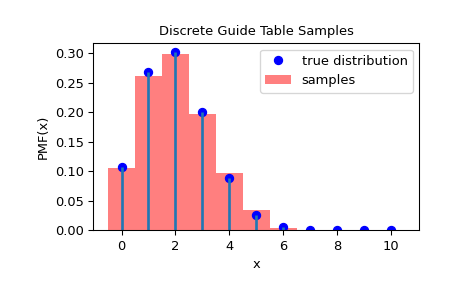
To check that the samples have been drawn from the correct distribution, we can visualize the histogram of the samples:

>>> import matplotlib.pyplot as plt
>>> rvs = rng.rvs(1000)
>>> fig = plt.figure()
>>> ax = fig.add_subplot(111)
>>> x = np.arange(0, n+1)
>>> fx = dist.pmf(x)
>>> fx = fx / fx.sum()
>>> ax.plot(x, fx, 'bo', label='true distribution')
>>> ax.vlines(x, 0, fx, lw=2)
>>> ax.hist(rvs, bins=np.r_[x, n+1]-0.5, density=True, alpha=0.5,
...         color='r', label='samples')
>>> ax.set_xlabel('x')
>>> ax.set_ylabel('PMF(x)')
>>> ax.set_title('Discrete Guide Table Samples')
>>> plt.legend()
>>> plt.show()

../../_images/scipy-stats-sampling-DiscreteGuideTable-1_00_00.png

To set the size of the guide table use the guide_factor keyword argument. This sets the size of the guide table relative to the probability vector

>>> rng = DiscreteGuideTable(pv, guide_factor=1, random_state=urng)

To calculate the PPF of a binomial distribution with \(n=4\) and \(p=0.1\): we can set up a guide table as follows:

>>> n, p = 4, 0.1
>>> dist = binom(n, p)
>>> rng = DiscreteGuideTable(dist, random_state=42)
>>> rng.ppf(0.5)
0.0

Methods

`ppf`(u)	PPF of the given distribution.
`rvs`([size, random_state])	Sample from the distribution.
`set_random_state`([random_state])	Set the underlying uniform random number generator.