scipy.stats.normal_inverse_gamma#

scipy.stats.normal_inverse_gamma = <scipy.stats._multivariate.normal_inverse_gamma_gen object>[source]#

Normal-inverse-gamma distribution.

The normal-inverse-gamma distribution is the conjugate prior of a normal distribution with unknown mean and variance.

Parameters:

mu, lmbda, a, barray_like: Shape parameters of the distribution. See notes.
seed{None, int, np.random.RandomState, np.random.Generator}, optional: Used for drawing random variates. If seed is None, the RandomState singleton is used. If seed is an int, a new RandomState instance is used, seeded with seed. If seed is already a RandomState or Generator instance, then that object is used. Default is None.

Methods

pdf(x, s2, mu=0, lmbda=1, a=1, b=1)	Probability density function.
logpdf(x, s2, mu=0, lmbda=1, a=1, b=1)	Log of the probability density function.
mean(mu=0, lmbda=1, a=1, b=1)	Distribution mean.
var(mu=0, lmbda=1, a=1, b=1)	Distribution variance.
rvs(mu=0, lmbda=1, a=1, b=1, size=None, random_state=None)	Draw random samples.

See also

norm
invgamma

Notes

The probability density function of normal_inverse_gamma is:

\[f(x, \sigma^2; \mu, \lambda, \alpha, \beta) = \frac{\sqrt{\lambda}}{\sqrt{2 \pi \sigma^2}} \frac{\beta^\alpha}{\Gamma(\alpha)} \left( \frac{1}{\sigma^2} \right)^{\alpha + 1} \exp \left(- \frac{2 \beta + \lambda (x - \mu)^2} {2 \sigma^2} \right)\]

where all parameters are real and finite, and \(\sigma^2 > 0\), \(\lambda > 0\), \(\alpha > 0\), and \(\beta > 0\).

Methods normal_inverse_gamma.pdf and normal_inverse_gamma.logpdf accept x and s2 for arguments \(x\) and \(\sigma^2\). All methods accept mu, lmbda, a, and b for shape parameters \(\mu\), \(\lambda\), \(\alpha\), and \(\beta\), respectively.

Added in version 1.15.

References

[1]

Normal-inverse-gamma distribution, Wikipedia, https://en.wikipedia.org/wiki/Normal-inverse-gamma_distribution

Examples

Suppose we wish to investigate the relationship between the normal-inverse-gamma distribution and the inverse gamma distribution.

>>> import numpy as np
>>> from scipy import stats
>>> import matplotlib.pyplot as plt
>>> rng = np.random.default_rng()
>>> mu, lmbda, a, b = 0, 1, 20, 20
>>> norm_inv_gamma = stats.normal_inverse_gamma(mu, lmbda, a, b)
>>> inv_gamma = stats.invgamma(a, scale=b)

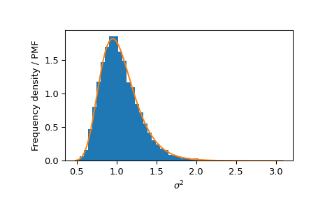
One approach is to compare the distribution of the s2 elements of random variates against the PDF of an inverse gamma distribution.

>>> _, s2 = norm_inv_gamma.rvs(size=10000, random_state=rng)
>>> bins = np.linspace(s2.min(), s2.max(), 50)
>>> plt.hist(s2, bins=bins, density=True, label='Frequency density')
>>> s2 = np.linspace(s2.min(), s2.max(), 300)
>>> plt.plot(s2, inv_gamma.pdf(s2), label='PDF')
>>> plt.xlabel(r'$\sigma^2$')
>>> plt.ylabel('Frequency density / PMF')
>>> plt.show()

../../_images/scipy-stats-normal_inverse_gamma-1_00_00.png

Similarly, we can compare the marginal distribution of s2 against an inverse gamma distribution.

>>> from scipy.integrate import quad_vec
>>> from scipy import integrate
>>> s2 = np.linspace(0.5, 3, 6)
>>> res = quad_vec(lambda x: norm_inv_gamma.pdf(x, s2), -np.inf, np.inf)[0]
>>> np.allclose(res, inv_gamma.pdf(s2))
True

The sample mean is comparable to the mean of the distribution.

>>> x, s2 = norm_inv_gamma.rvs(size=10000, random_state=rng)
>>> x.mean(), s2.mean()
(np.float64(-0.005254750127304425), np.float64(1.050438111436508))
>>> norm_inv_gamma.mean()
(np.float64(0.0), np.float64(1.0526315789473684))

Similarly, for the variance:

>>> x.var(ddof=1), s2.var(ddof=1)
(np.float64(1.0546150578185023), np.float64(0.061829865266330754))
>>> norm_inv_gamma.var()
(np.float64(1.0526315789473684), np.float64(0.061557402277623886))