scipy.stats.

gaussian_kde#

class scipy.stats.gaussian_kde(dataset, bw_method=None, weights=None)[source]#

Representation of a kernel-density estimate using Gaussian kernels.

Kernel density estimation is a way to estimate the probability density function (PDF) of a random variable in a non-parametric way. gaussian_kde works for both uni-variate and multi-variate data. It includes automatic bandwidth determination. The estimation works best for a unimodal distribution; bimodal or multi-modal distributions tend to be oversmoothed.

Parameters:

datasetarray_like: Datapoints to estimate from. In case of univariate data this is a 1-D array, otherwise a 2-D array with shape (# of dims, # of data).
bw_methodstr, scalar or callable, optional: The method used to calculate the bandwidth factor. This can be ‘scott’, ‘silverman’, a scalar constant or a callable. If a scalar, this will be used directly as factor. If a callable, it should take a gaussian_kde instance as only parameter and return a scalar. If None (default), ‘scott’ is used. See Notes for more details.
weightsarray_like, optional: weights of datapoints. This must be the same shape as dataset. If None (default), the samples are assumed to be equally weighted

Attributes:

datasetndarray: The dataset with which gaussian_kde was initialized.
dint: Number of dimensions.
nint: Number of datapoints.
neffint: Effective number of datapoints.

Added in version 1.2.0.
factorfloat: The bandwidth factor obtained from covariance_factor.
covariancendarray: The kernel covariance matrix; this is the data covariance matrix multiplied by the square of the bandwidth factor, e.g. np.cov(dataset) * factor**2.
inv_covndarray: The inverse of covariance.

Methods

`evaluate`(points)	Evaluate the estimated pdf on a set of points.
`__call__`(points)	Evaluate the estimated pdf on a set of points.
`integrate_gaussian`(mean, cov)	Multiply estimated density by a multivariate Gaussian and integrate over the whole space.
`integrate_box_1d`(low, high)	Computes the integral of a 1D pdf between two bounds.
`integrate_box`(low_bounds, high_bounds[, ...])	Computes the integral of a pdf over a rectangular interval.
`integrate_kde`(other)	Computes the integral of the product of this kernel density estimate with another.
`pdf`(x)	Evaluate the estimated pdf on a provided set of points.
`logpdf`(x)	Evaluate the log of the estimated pdf on a provided set of points.
`resample`([size, seed])	Randomly sample a dataset from the estimated pdf.
`set_bandwidth`([bw_method])	Compute the bandwidth factor with given method.
`covariance_factor`()	Computes the bandwidth factor factor.

Notes

Bandwidth selection strongly influences the estimate obtained from the KDE (much more so than the actual shape of the kernel). Bandwidth selection can be done by a “rule of thumb”, by cross-validation, by “plug-in methods” or by other means; see [3], [4] for reviews. gaussian_kde uses a rule of thumb, the default is Scott’s Rule.

Scott’s Rule [1], implemented as scotts_factor, is:

n**(-1./(d+4)),

with n the number of data points and d the number of dimensions. In the case of unequally weighted points, scotts_factor becomes:

neff**(-1./(d+4)),

with neff the effective number of datapoints. Silverman’s suggestion for multivariate data [2], implemented as silverman_factor, is:

(n * (d + 2) / 4.)**(-1. / (d + 4)).

or in the case of unequally weighted points:

(neff * (d + 2) / 4.)**(-1. / (d + 4)).

Note that this is not the same as “Silverman’s rule of thumb” [6], which may be more robust in the univariate case; see documentation of the set_bandwidth method for implementing a custom bandwidth rule.

Good general descriptions of kernel density estimation can be found in [1] and [2], the mathematics for this multi-dimensional implementation can be found in [1].

With a set of weighted samples, the effective number of datapoints neff is defined by:

neff = sum(weights)^2 / sum(weights^2)

as detailed in [5].

gaussian_kde does not currently support data that lies in a lower-dimensional subspace of the space in which it is expressed. For such data, consider performing principal component analysis / dimensionality reduction and using gaussian_kde with the transformed data.

References

[1] (1,2,3)

D.W. Scott, “Multivariate Density Estimation: Theory, Practice, and Visualization”, John Wiley & Sons, New York, Chicester, 1992.

[2] (1,2)

B.W. Silverman, “Density Estimation for Statistics and Data Analysis”, Vol. 26, Monographs on Statistics and Applied Probability, Chapman and Hall, London, 1986.

[3]

B.A. Turlach, “Bandwidth Selection in Kernel Density Estimation: A Review”, CORE and Institut de Statistique, Vol. 19, pp. 1-33, 1993.

[4]

D.M. Bashtannyk and R.J. Hyndman, “Bandwidth selection for kernel conditional density estimation”, Computational Statistics & Data Analysis, Vol. 36, pp. 279-298, 2001.

[5]

Gray P. G., 1969, Journal of the Royal Statistical Society. Series A (General), 132, 272

[6]

Kernel density estimation. Wikipedia. https://en.wikipedia.org/wiki/Kernel_density_estimation

Examples

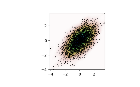
Generate some random two-dimensional data:

>>> import numpy as np
>>> from scipy import stats
>>> def measure(n):
...     "Measurement model, return two coupled measurements."
...     m1 = np.random.normal(size=n)
...     m2 = np.random.normal(scale=0.5, size=n)
...     return m1+m2, m1-m2

>>> m1, m2 = measure(2000)
>>> xmin = m1.min()
>>> xmax = m1.max()
>>> ymin = m2.min()
>>> ymax = m2.max()

Perform a kernel density estimate on the data:

>>> X, Y = np.mgrid[xmin:xmax:100j, ymin:ymax:100j]
>>> positions = np.vstack([X.ravel(), Y.ravel()])
>>> values = np.vstack([m1, m2])
>>> kernel = stats.gaussian_kde(values)
>>> Z = np.reshape(kernel(positions).T, X.shape)

Plot the results:

>>> import matplotlib.pyplot as plt
>>> fig, ax = plt.subplots()
>>> ax.imshow(np.rot90(Z), cmap=plt.cm.gist_earth_r,
...           extent=[xmin, xmax, ymin, ymax])
>>> ax.plot(m1, m2, 'k.', markersize=2)
>>> ax.set_xlim([xmin, xmax])
>>> ax.set_ylim([ymin, ymax])
>>> plt.show()

../../_images/scipy-stats-gaussian_kde-1_00_00.png

Compare against manual KDE at a point:

>>> point = [1, 2]
>>> mean = values.T
>>> cov = kernel.factor**2 * np.cov(values)
>>> X = stats.multivariate_normal(cov=cov)
>>> res = kernel.pdf(point)
>>> ref = X.pdf(point - mean).sum() / len(mean)
>>> np.allclose(res, ref)
True