boxcox_llf#

scipy.stats.boxcox_llf(lmb, data, *, axis=0, keepdims=False, nan_policy='propagate')[source]#

The boxcox log-likelihood function.

Parameters:

lmbscalar

Parameter for Box-Cox transformation. See boxcox for details.

dataarray_like

Data to calculate Box-Cox log-likelihood for. If data is multi-dimensional, the log-likelihood is calculated along the first axis.

axisint, default: 0

If an int, the axis of the input along which to compute the statistic. The statistic of each axis-slice (e.g. row) of the input will appear in a corresponding element of the output. If None, the input will be raveled before computing the statistic.

nan_policy{‘propagate’, ‘omit’, ‘raise’

Defines how to handle input NaNs.

• propagate: if a NaN is present in the axis slice (e.g. row) along which the statistic is computed, the corresponding entry of the output will be NaN.

• omit: NaNs will be omitted when performing the calculation. If insufficient data remains in the axis slice along which the statistic is computed, the corresponding entry of the output will be NaN.

• raise: if a NaN is present, a ValueError will be raised.

keepdimsbool, default: False

If this is set to True, the axes which are reduced are left in the result as dimensions with size one. With this option, the result will broadcast correctly against the input array.

Returns:

llffloat or ndarray

Box-Cox log-likelihood of data given lmb. A float for 1-D data, an array otherwise.

See also

boxcox, probplot, boxcox_normplot, boxcox_normmax

Notes

The Box-Cox log-likelihood function \(l\) is defined here as

\[l = (\lambda - 1) \sum_i^N \log(x_i) - \frac{N}{2} \log\left(\sum_i^N (y_i - \bar{y})^2 / N\right),\]

where \(N\) is the number of data points data and \(y\) is the Box-Cox transformed input data. This corresponds to the profile log-likelihood of the original data \(x\) with some constant terms dropped.

Examples

Try it in your browser!

>>> import numpy as np
>>> from scipy import stats
>>> import matplotlib.pyplot as plt
>>> from mpl_toolkits.axes_grid1.inset_locator import inset_axes

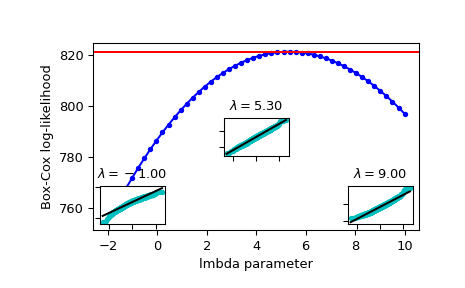
Generate some random variates and calculate Box-Cox log-likelihood values for them for a range of lmbda values:

>>> rng = np.random.default_rng()
>>> x = stats.loggamma.rvs(5, loc=10, size=1000, random_state=rng)
>>> lmbdas = np.linspace(-2, 10)
>>> llf = np.zeros(lmbdas.shape, dtype=float)
>>> for ii, lmbda in enumerate(lmbdas):
...     llf[ii] = stats.boxcox_llf(lmbda, x)

Also find the optimal lmbda value with boxcox:

>>> x_most_normal, lmbda_optimal = stats.boxcox(x)

Plot the log-likelihood as function of lmbda. Add the optimal lmbda as a horizontal line to check that that’s really the optimum:

>>> fig = plt.figure()
>>> ax = fig.add_subplot(111)
>>> ax.plot(lmbdas, llf, 'b.-')
>>> ax.axhline(stats.boxcox_llf(lmbda_optimal, x), color='r')
>>> ax.set_xlabel('lmbda parameter')
>>> ax.set_ylabel('Box-Cox log-likelihood')

Now add some probability plots to show that where the log-likelihood is maximized the data transformed with boxcox looks closest to normal:

>>> locs = [3, 10, 4]  # 'lower left', 'center', 'lower right'
>>> for lmbda, loc in zip([-1, lmbda_optimal, 9], locs):
...     xt = stats.boxcox(x, lmbda=lmbda)
...     (osm, osr), (slope, intercept, r_sq) = stats.probplot(xt)
...     ax_inset = inset_axes(ax, width="20%", height="20%", loc=loc)
...     ax_inset.plot(osm, osr, 'c.', osm, slope*osm + intercept, 'k-')
...     ax_inset.set_xticklabels([])
...     ax_inset.set_yticklabels([])
...     ax_inset.set_title(r'$\lambda=%1.2f$' % lmbda)

>>> plt.show()

Go BackOpen In Tab