scipy.special.y1#

scipy.special.y1(x, out=None) = <ufunc 'y1'>#

Bessel function of the second kind of order 1.

Parameters:

xarray_like: Argument (float).
outndarray, optional: Optional output array for the function results

Returns:

Yscalar or ndarray: Value of the Bessel function of the second kind of order 1 at x.

See also

j1: Bessel function of the first kind of order 1
yn: Bessel function of the second kind
yv: Bessel function of the second kind

Notes

The domain is divided into the intervals [0, 8] and (8, infinity). In the first interval a 25 term Chebyshev expansion is used, and computing \(J_1\) (the Bessel function of the first kind) is required. In the second, the asymptotic trigonometric representation is employed using two rational functions of degree 5/5.

This function is a wrapper for the Cephes [1] routine y1.

Array API Standard Support

y1 has support for Python Array API Standard compatible backends in addition to NumPy. The following combinations of backend and device (or other capability) are supported.

Library	CPU	GPU
NumPy	✅	n/a
CuPy	n/a	✅
PyTorch	✅	✅
JAX	✅	⛔
Dask	✅	n/a

For the NumPy backend, this function supports all NumPy ufunc keyword arguments. Other backends may support out, but none of the other ufunc kwargs. out is typically supported for CuPy and PyTorch, but not currently in cases where SciPy relies on a generic Array API implementation or, for PyTorch on CPU, falls back to the NumPy backend. out is never supported for JAX because JAX arrays are immutable.

See Support for the array API standard for more information.

References

[1]

Cephes Mathematical Functions Library, http://www.netlib.org/cephes/

Examples

Calculate the function at one point:

>>> from scipy.special import y1
>>> y1(1.)
-0.7812128213002888

Calculate at several points:

>>> import numpy as np
>>> y1(np.array([0.5, 2., 3.]))
array([-1.47147239, -0.10703243,  0.32467442])

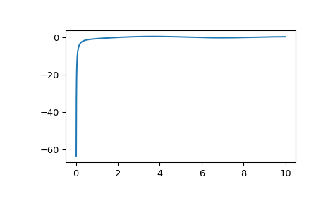
Plot the function from 0 to 10.

>>> import matplotlib.pyplot as plt
>>> fig, ax = plt.subplots()
>>> x = np.linspace(0., 10., 1000)
>>> y = y1(x)
>>> ax.plot(x, y)
>>> plt.show()