scipy.special.hankel1#

scipy.special.hankel1(v, z, out=None) = <wrapped_ufunc 'hankel1'>#

Hankel function of the first kind.

Parameters:

varray_like: Order (float).
zarray_like: Argument (float or complex).
outndarray, optional: Optional output array for the function values

Returns:

scalar or ndarray: Values of the Hankel function of the first kind.

See also

hankel1e: This function with leading exponential behavior stripped off.

Notes

A wrapper for the AMOS [1] routine zbesh, which carries out the computation using the relation,

\[H^{(1)}_v(z) = \frac{2}{\imath\pi} \exp(-\imath \pi v/2) K_v(z \exp(-\imath\pi/2))\]

where \(K_v\) is the modified Bessel function of the second kind. For negative orders, the relation

\[H^{(1)}_{-v}(z) = H^{(1)}_v(z) \exp(\imath\pi v)\]

is used.

Array API Standard Support

hankel1 has support for Python Array API Standard compatible backends in addition to NumPy. The following combinations of backend and device (or other capability) are supported.

Library	CPU	GPU
NumPy	✅	n/a
CuPy	n/a	⛔
PyTorch	✅	⛔
JAX	✅	⛔
Dask	✅	n/a

For the NumPy backend, this function supports all NumPy ufunc keyword arguments. Other backends may support out, but typically none of the other ufunc kwargs. out is typically supported for CuPy and PyTorch, but not currently in cases where SciPy relies on a generic Array API implementation or, for PyTorch on CPU, falls back to the NumPy backend. out is never supported for JAX because JAX arrays are immutable. hankel1 does not currently support out for the PyTorch backend.

See Support for the array API standard for more information.

References

[1]

Donald E. Amos, “AMOS, A Portable Package for Bessel Functions of a Complex Argument and Nonnegative Order”, http://netlib.org/amos/

Examples

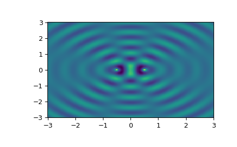
For the inhomogeneous Helmholtz equation in \(\mathbb{R}^2\) subject to radiation boundary conditions, the Green’s function is given by

\[G(\mathbf{x}, \mathbf{x}^\prime) = \frac{1}{4i} H^{(1)}_0(k|\mathbf{x} - \mathbf{x^\prime}|)\]

where \(k\) is the wavenumber and \(H^{(1)}_0\) is the Hankel function of the first kind and of order zero. In the following example, we will solve the Helmholtz equation with two Dirac sources.

>>> import numpy as np
>>> import matplotlib.pyplot as plt
>>> from scipy.special import hankel1
>>> k = 10  # Wavenumber
>>> sources = [0.5, -0.5]  # Location of two point sources
>>> x, y = np.linspace(-3, 3, 300), np.linspace(-3, 3, 300)
>>> Z = np.add.outer(1j*y, x)
>>> U = np.zeros_like(Z)
>>> for sz in sources:
...     r = np.abs(Z - sz)
...     U += (1j/4)*hankel1(0, k*r)

Finally, we will plot the real part of the solution.

>>> fig, ax = plt.subplots()
>>> ax.pcolormesh(np.real(Z), np.imag(Z), np.real(U))
>>> plt.show()

../../_images/scipy-special-hankel1-1.png