scipy.special.fdtri

scipy.special.fdtri(dfn, dfd, p, out=None) = <ufunc 'fdtri'>

The p-th quantile of the F-distribution.

This function is the inverse of the F-distribution CDF, fdtr, returning the x such that fdtr(dfn, dfd, x) = p.

Parameters:

dfnarray_like

First parameter (positive float).

dfdarray_like

Second parameter (positive float).

parray_like

Cumulative probability, in [0, 1].

outndarray, optional

Optional output array for the function values

Returns:

xscalar or ndarray

The quantile corresponding to p.

See also

fdtr

F distribution cumulative distribution function

fdtrc

F distribution survival function

scipy.stats.f

F distribution

Notes

Wrapper for a routine from the Boost Math C++ library [1]. The F distribution is also available as scipy.stats.f. Calling fdtri directly can improve performance compared to the ppf method of scipy.stats.f (see last example below).

Array API Standard Support

fdtri has experimental support for Python Array API Standard compatible backends in addition to NumPy. Please consider testing these features by setting an environment variable SCIPY_ARRAY_API=1 and providing CuPy, PyTorch, JAX, or Dask arrays as array arguments. The following combinations of backend and device (or other capability) are supported.

Library	CPU	GPU
NumPy	✅	n/a
CuPy	n/a	✅
PyTorch	✅	⛔
JAX	⚠️ no JIT	⛔
Dask	✅	n/a

See Support for the array API standard for more information.

References

[1]

The Boost Developers. “Boost C++ Libraries”. https://www.boost.org/.

Examples

Try it in your browser!

fdtri represents the inverse of the F distribution CDF which is available as fdtr. Here, we calculate the CDF for df1=1, df2=2 at x=3. fdtri then returns 3 given the same values for df1, df2 and the computed CDF value.

>>> import numpy as np
>>> from scipy.special import fdtri, fdtr
>>> df1, df2 = 1, 2
>>> x = 3
>>> cdf_value =  fdtr(df1, df2, x)
>>> fdtri(df1, df2, cdf_value)
3.000000000000006

Calculate the function at several points by providing a NumPy array for x.

>>> x = np.array([0.1, 0.4, 0.7])
>>> fdtri(1, 2, x)
array([0.02020202, 0.38095238, 1.92156863])

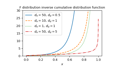
Plot the function for several parameter sets.

>>> import matplotlib.pyplot as plt
>>> dfn_parameters = [50, 10, 1, 50]
>>> dfd_parameters = [0.5, 1, 1, 5]
>>> linestyles = ['solid', 'dashed', 'dotted', 'dashdot']
>>> parameters_list = list(zip(dfn_parameters, dfd_parameters,
...                            linestyles))
>>> x = np.linspace(0, 1, 1000)
>>> fig, ax = plt.subplots()
>>> for parameter_set in parameters_list:
...     dfn, dfd, style = parameter_set
...     fdtri_vals = fdtri(dfn, dfd, x)
...     ax.plot(x, fdtri_vals, label=rf"$d_n={dfn},\, d_d={dfd}$",
...             ls=style)
>>> ax.legend()
>>> ax.set_xlabel("$x$")
>>> title = "F distribution inverse cumulative distribution function"
>>> ax.set_title(title)
>>> ax.set_ylim(0, 30)
>>> plt.show()

The F distribution is also available as scipy.stats.f. Using fdtri directly can be much faster than calling the ppf method of scipy.stats.f, especially for small arrays or individual values. To get the same results one must use the following parametrization: stats.f(dfn, dfd).ppf(x)=fdtri(dfn, dfd, x).

>>> from scipy.stats import f
>>> dfn, dfd = 1, 2
>>> x = 0.7
>>> fdtri_res = fdtri(dfn, dfd, x)  # this will often be faster than below
>>> f_dist_res = f(dfn, dfd).ppf(x)
>>> f_dist_res == fdtri_res  # test that results are equal
True

Go BackOpen In Tab