scipy.signal.

lfilter#

scipy.signal.lfilter(b, a, x, axis=-1, zi=None)[source]#

Filter data along one-dimension with an IIR or FIR filter.

Filter a data sequence, x, using a digital filter. This works for many fundamental data types (including Object type). The filter is a direct form II transposed implementation of the standard difference equation (see Notes).

The function sosfilt (and filter design using output='sos') should be preferred over lfilter for most filtering tasks, as second-order sections have fewer numerical problems.

Parameters:

barray_like: The numerator coefficient vector in a 1-D sequence.
aarray_like: The denominator coefficient vector in a 1-D sequence. If a[0] is not 1, then both a and b are normalized by a[0].
xarray_like: An N-dimensional input array.
axisint, optional: The axis of the input data array along which to apply the linear filter. The filter is applied to each subarray along this axis. Default is -1.
ziarray_like, optional: Initial conditions for the filter delays. It is a vector (or array of vectors for an N-dimensional input) of length max(len(a), len(b)) - 1. If zi is None or is not given then initial rest is assumed. See lfiltic for more information.

Returns:

yarray: The output of the digital filter.
zfarray, optional: If zi is None, this is not returned, otherwise, zf holds the final filter delay values.

See also

lfiltic: Construct initial conditions for lfilter.
lfilter_zi: Compute initial state (steady state of step response) for lfilter.
filtfilt: A forward-backward filter, to obtain a filter with zero phase.
savgol_filter: A Savitzky-Golay filter.
sosfilt: Filter data using cascaded second-order sections.
sosfiltfilt: A forward-backward filter using second-order sections.

Notes

The filter function is implemented as a direct II transposed structure. This means that the filter implements:

a[0]*y[n] = b[0]*x[n] + b[1]*x[n-1] + ... + b[M]*x[n-M]
                      - a[1]*y[n-1] - ... - a[N]*y[n-N]

where M is the degree of the numerator, N is the degree of the denominator, and n is the sample number. It is implemented using the following difference equations (assuming M = N):

a[0]*y[n] = b[0] * x[n]               + d[0][n-1]
  d[0][n] = b[1] * x[n] - a[1] * y[n] + d[1][n-1]
  d[1][n] = b[2] * x[n] - a[2] * y[n] + d[2][n-1]
...
d[N-2][n] = b[N-1]*x[n] - a[N-1]*y[n] + d[N-1][n-1]
d[N-1][n] = b[N] * x[n] - a[N] * y[n]

where d are the state variables.

The rational transfer function describing this filter in the z-transform domain is:

                    -1              -M
        b[0] + b[1]z  + ... + b[M] z
Y(z) = -------------------------------- X(z)
                    -1              -N
        a[0] + a[1]z  + ... + a[N] z

Array API Standard Support

lfilter has support for Python Array API Standard compatible backends in addition to NumPy. The following combinations of backend and device (or other capability) are supported.

Library	CPU	GPU
NumPy	✅	n/a
CuPy	n/a	✅
PyTorch	✅	⛔
JAX	⚠️ no JIT	⛔
Dask	⚠️ computes graph	n/a

See Support for the array API standard for more information.

Examples

Generate a noisy signal to be filtered:

>>> import numpy as np
>>> from scipy import signal
>>> import matplotlib.pyplot as plt
>>> rng = np.random.default_rng()
>>> t = np.linspace(-1, 1, 201)
>>> x = (np.sin(2*np.pi*0.75*t*(1-t) + 2.1) +
...      0.1*np.sin(2*np.pi*1.25*t + 1) +
...      0.18*np.cos(2*np.pi*3.85*t))
>>> xn = x + rng.standard_normal(len(t)) * 0.08

Create an order 3 lowpass butterworth filter:

>>> b, a = signal.butter(3, 0.05)

Apply the filter to xn. Use lfilter_zi to choose the initial condition of the filter:

>>> zi = signal.lfilter_zi(b, a)
>>> z, _ = signal.lfilter(b, a, xn, zi=zi*xn[0])

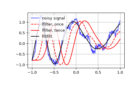
Apply the filter again, to have a result filtered at an order the same as filtfilt:

>>> z2, _ = signal.lfilter(b, a, z, zi=zi*z[0])

Use filtfilt to apply the filter:

>>> y = signal.filtfilt(b, a, xn)

Plot the original signal and the various filtered versions:

>>> plt.figure
>>> plt.plot(t, xn, 'b', alpha=0.75)
>>> plt.plot(t, z, 'r--', t, z2, 'r', t, y, 'k')
>>> plt.legend(('noisy signal', 'lfilter, once', 'lfilter, twice',
...             'filtfilt'), loc='best')
>>> plt.grid(True)
>>> plt.show()

../../_images/scipy-signal-lfilter-1.png