scipy.signal.

impulse#

scipy.signal.impulse(system, X0=None, T=None, N=None)[source]#

Impulse response of continuous-time system.

Parameters:

systeman instance of the LTI class or a tuple of array_like

describing the system. The following gives the number of elements in the tuple and the interpretation:

1 (instance of lti)

2 (num, den)

3 (zeros, poles, gain)

4 (A, B, C, D)

X0array_like, optional

Initial state-vector. Defaults to zero.

Tarray_like, optional

Time points. Computed if not given.

Nint, optional

The number of time points to compute (if T is not given).

Returns:

Tndarray: A 1-D array of time points.
youtndarray: A 1-D array containing the impulse response of the system (except for singularities at zero).

Notes

If (num, den) is passed in for system, coefficients for both the numerator and denominator should be specified in descending exponent order (e.g. s^2 + 3s + 5 would be represented as [1, 3, 5]).

Array API Standard Support

impulse has experimental support for Python Array API Standard compatible backends in addition to NumPy. Please consider testing these features by setting an environment variable SCIPY_ARRAY_API=1 and providing CuPy, PyTorch, JAX, or Dask arrays as array arguments. The following combinations of backend and device (or other capability) are supported.

Library	CPU	GPU
NumPy	✅	n/a
CuPy	n/a	✅
PyTorch	✅	✅
JAX	✅	✅
Dask	✅	n/a

See Support for the array API standard for more information.

Examples

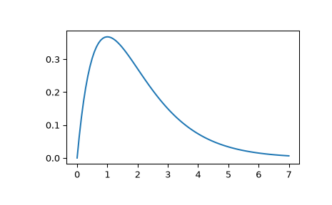
Compute the impulse response of a second order system with a repeated root: x''(t) + 2*x'(t) + x(t) = u(t)

>>> from scipy import signal
>>> system = ([1.0], [1.0, 2.0, 1.0])
>>> t, y = signal.impulse(system)
>>> import matplotlib.pyplot as plt
>>> plt.plot(t, y)

../../_images/scipy-signal-impulse-1.png