scipy.signal.correlate

scipy.signal.correlate(in1, in2, mode='full', method='auto')

Cross-correlate two N-dimensional arrays.

Cross-correlate in1 and in2, with the output size determined by the mode argument.

Parameters:

in1array_like

First input.

in2array_like

Second input. Should have the same number of dimensions as in1.

modestr {‘full’, ‘valid’, ‘same’}, optional

A string indicating the size of the output:

full

The output is the full discrete linear cross-correlation of the inputs. (Default)

valid

The output consists only of those elements that do not rely on the zero-padding. In ‘valid’ mode, either in1 or in2 must be at least as large as the other in every dimension.

same

The output is the same size as in1, centered with respect to the ‘full’ output.

methodstr {‘auto’, ‘direct’, ‘fft’}, optional

A string indicating which method to use to calculate the correlation.

direct

The correlation is determined directly from sums, the definition of correlation.

fft

The Fast Fourier Transform is used to perform the correlation more quickly (only available for numerical arrays.)

auto

Automatically chooses direct or Fourier method based on an estimate of which is faster (default). See convolve Notes for more detail.

New in version 0.19.0.

Returns:

correlatearray

An N-dimensional array containing a subset of the discrete linear cross-correlation of in1 with in2.

See also

choose_conv_method

contains more documentation on method.

correlation_lags

calculates the lag / displacement indices array for 1D cross-correlation.

Notes

The correlation z of two d-dimensional arrays x and y is defined as:

z[...,k,...] = sum[..., i_l, ...] x[..., i_l,...] * conj(y[..., i_l - k,...])

This way, if x and y are 1-D arrays and z = correlate(x, y, 'full') then

\[z[k] = (x * y)(k - N + 1) = \sum_{l=0}^{||x||-1}x_l y_{l-k+N-1}^{*}\]

for \(k = 0, 1, ..., ||x|| + ||y|| - 2\)

where \(||x||\) is the length of x, \(N = \max(||x||,||y||)\), and \(y_m\) is 0 when m is outside the range of y.

method='fft' only works for numerical arrays as it relies on fftconvolve. In certain cases (i.e., arrays of objects or when rounding integers can lose precision), method='direct' is always used.

When using “same” mode with even-length inputs, the outputs of correlate and correlate2d differ: There is a 1-index offset between them.

Examples

Try it in your browser!

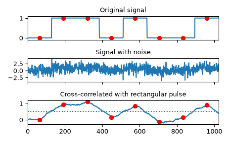
Implement a matched filter using cross-correlation, to recover a signal that has passed through a noisy channel.

>>> import numpy as np
>>> from scipy import signal
>>> import matplotlib.pyplot as plt
>>> rng = np.random.default_rng()

>>> sig = np.repeat([0., 1., 1., 0., 1., 0., 0., 1.], 128)
>>> sig_noise = sig + rng.standard_normal(len(sig))
>>> corr = signal.correlate(sig_noise, np.ones(128), mode='same') / 128

>>> clock = np.arange(64, len(sig), 128)
>>> fig, (ax_orig, ax_noise, ax_corr) = plt.subplots(3, 1, sharex=True)
>>> ax_orig.plot(sig)
>>> ax_orig.plot(clock, sig[clock], 'ro')
>>> ax_orig.set_title('Original signal')
>>> ax_noise.plot(sig_noise)
>>> ax_noise.set_title('Signal with noise')
>>> ax_corr.plot(corr)
>>> ax_corr.plot(clock, corr[clock], 'ro')
>>> ax_corr.axhline(0.5, ls=':')
>>> ax_corr.set_title('Cross-correlated with rectangular pulse')
>>> ax_orig.margins(0, 0.1)
>>> fig.tight_layout()
>>> plt.show()

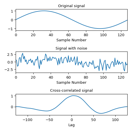
Compute the cross-correlation of a noisy signal with the original signal.

>>> x = np.arange(128) / 128
>>> sig = np.sin(2 * np.pi * x)
>>> sig_noise = sig + rng.standard_normal(len(sig))
>>> corr = signal.correlate(sig_noise, sig)
>>> lags = signal.correlation_lags(len(sig), len(sig_noise))
>>> corr /= np.max(corr)

>>> fig, (ax_orig, ax_noise, ax_corr) = plt.subplots(3, 1, figsize=(4.8, 4.8))
>>> ax_orig.plot(sig)
>>> ax_orig.set_title('Original signal')
>>> ax_orig.set_xlabel('Sample Number')
>>> ax_noise.plot(sig_noise)
>>> ax_noise.set_title('Signal with noise')
>>> ax_noise.set_xlabel('Sample Number')
>>> ax_corr.plot(lags, corr)
>>> ax_corr.set_title('Cross-correlated signal')
>>> ax_corr.set_xlabel('Lag')
>>> ax_orig.margins(0, 0.1)
>>> ax_noise.margins(0, 0.1)
>>> ax_corr.margins(0, 0.1)
>>> fig.tight_layout()
>>> plt.show()

Go BackOpen In Tab