scipy.signal.

convolve2d#

scipy.signal.convolve2d(in1, in2, mode='full', boundary='fill', fillvalue=0)[source]#

Convolve two 2-dimensional arrays.

Convolve in1 and in2 with output size determined by mode, and boundary conditions determined by boundary and fillvalue.

Parameters:

in1array_like

First input.

in2array_like

Second input. Should have the same number of dimensions as in1.

modestr {‘full’, ‘valid’, ‘same’}, optional

A string indicating the size of the output:

full: The output is the full discrete linear convolution of the inputs. (Default)
valid: The output consists only of those elements that do not rely on the zero-padding. In ‘valid’ mode, either in1 or in2 must be at least as large as the other in every dimension.
same: The output is the same size as in1, centered with respect to the ‘full’ output.

boundarystr {‘fill’, ‘wrap’, ‘symm’}, optional

A flag indicating how to handle boundaries:

fill: pad input arrays with fillvalue. (default)
wrap: circular boundary conditions.
symm: symmetrical boundary conditions.

fillvaluescalar, optional

Value to fill pad input arrays with. Default is 0.

Returns:

outndarray: A 2-dimensional array containing a subset of the discrete linear convolution of in1 with in2.

Notes

Array API Standard Support

convolve2d has experimental support for Python Array API Standard compatible backends in addition to NumPy. Please consider testing these features by setting an environment variable SCIPY_ARRAY_API=1 and providing CuPy, PyTorch, JAX, or Dask arrays as array arguments. The following combinations of backend and device (or other capability) are supported.

Library	CPU	GPU
NumPy	✅	n/a
CuPy	n/a	✅
PyTorch	✅	⛔
JAX	✅	✅
Dask	⚠️ computes graph	n/a

The JAX backend only supports boundary="fill" and fillvalue=0.

See Support for the array API standard for more information.

Examples

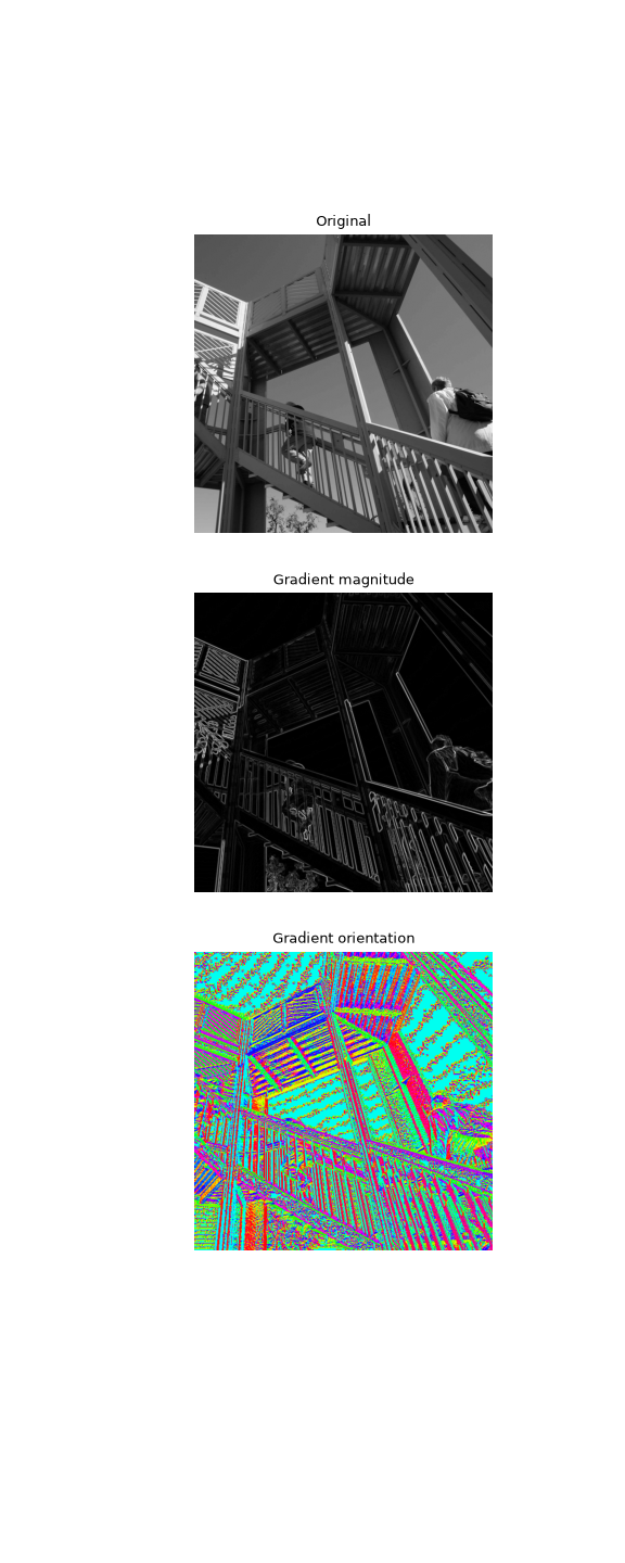
Compute the gradient of an image by 2D convolution with a complex Scharr operator. (Horizontal operator is real, vertical is imaginary.) Use symmetric boundary condition to avoid creating edges at the image boundaries.

>>> import numpy as np
>>> from scipy import signal
>>> from scipy import datasets
>>> ascent = datasets.ascent()
>>> scharr = np.array([[ -3-3j, 0-10j,  +3 -3j],
...                    [-10+0j, 0+ 0j, +10 +0j],
...                    [ -3+3j, 0+10j,  +3 +3j]]) # Gx + j*Gy
>>> grad = signal.convolve2d(ascent, scharr, boundary='symm', mode='same')

>>> import matplotlib.pyplot as plt
>>> fig, (ax_orig, ax_mag, ax_ang) = plt.subplots(3, 1, figsize=(6, 15))
>>> ax_orig.imshow(ascent, cmap='gray')
>>> ax_orig.set_title('Original')
>>> ax_orig.set_axis_off()
>>> ax_mag.imshow(np.absolute(grad), cmap='gray')
>>> ax_mag.set_title('Gradient magnitude')
>>> ax_mag.set_axis_off()
>>> ax_ang.imshow(np.angle(grad), cmap='hsv') # hsv is cyclic, like angles
>>> ax_ang.set_title('Gradient orientation')
>>> ax_ang.set_axis_off()
>>> fig.show()

../../_images/scipy-signal-convolve2d-1.png