chirp#
- scipy.signal.chirp(t, f0, t1, f1, method='linear', phi=0, vertex_zero=True, *, complex=False)[source]#
Frequency-swept cosine generator.
In the following, ‘Hz’ should be interpreted as ‘cycles per unit’; there is no requirement here that the unit is one second. The important distinction is that the units of rotation are cycles, not radians. Likewise, t could be a measurement of space instead of time.
- Parameters:
- tarray_like
Times at which to evaluate the waveform.
- f0float
Frequency (e.g. Hz) at time t=0.
- t1float
Time at which f1 is specified.
- f1float
Frequency (e.g. Hz) of the waveform at time t1.
- method{‘linear’, ‘quadratic’, ‘logarithmic’, ‘hyperbolic’}, optional
Kind of frequency sweep. If not given, linear is assumed. See Notes below for more details.
- phifloat, optional
Phase offset, in degrees. Default is 0.
- vertex_zerobool, optional
This parameter is only used when method is ‘quadratic’. It determines whether the vertex of the parabola that is the graph of the frequency is at t=0 or t=t1.
- complexbool, optional
This parameter creates a complex-valued analytic signal instead of a real-valued signal. It allows the use of complex baseband (in communications domain). Default is False.
Added in version 1.15.0.
- Returns:
- yndarray
A numpy array containing the signal evaluated at t with the requested time-varying frequency. More precisely, the function returns
exp(1j*phase + 1j*(pi/180)*phi) if complex else cos(phase + (pi/180)*phi)where phase is the integral (from 0 to t) of2*pi*f(t). The instantaneous frequencyf(t)is defined below.
See also
Notes
There are four possible options for the parameter method, which have a (long) standard form and some allowed abbreviations. The formulas for the instantaneous frequency \(f(t)\) of the generated signal are as follows:
Parameter method in
('linear', 'lin', 'li'):\[f(t) = f_0 + \beta\, t \quad\text{with}\quad \beta = \frac{f_1 - f_0}{t_1}\]Frequency \(f(t)\) varies linearly over time with a constant rate \(\beta\).
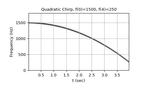
Parameter method in
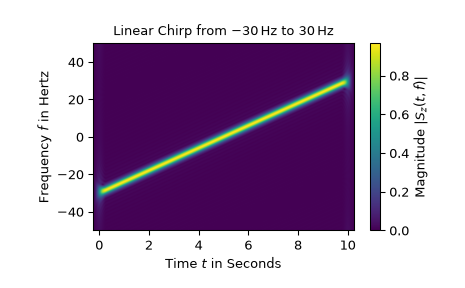
('quadratic', 'quad', 'q'):\[\begin{split}f(t) = \begin{cases} f_0 + \beta\, t^2 & \text{if vertex_zero is True,}\\ f_1 + \beta\, (t_1 - t)^2 & \text{otherwise,} \end{cases} \quad\text{with}\quad \beta = \frac{f_1 - f_0}{t_1^2}\end{split}\]The graph of the frequency f(t) is a parabola through \((0, f_0)\) and \((t_1, f_1)\). By default, the vertex of the parabola is at \((0, f_0)\). If vertex_zero is
False, then the vertex is at \((t_1, f_1)\). To use a more general quadratic function, or an arbitrary polynomial, use the functionscipy.signal.sweep_poly.Parameter method in
('logarithmic', 'log', 'lo'):\[f(t) = f_0 \left(\frac{f_1}{f_0}\right)^{t/t_1}\]\(f_0\) and \(f_1\) must be nonzero and have the same sign. This signal is also known as a geometric or exponential chirp.
Parameter method in
('hyperbolic', 'hyp'):\[f(t) = \frac{\alpha}{\beta\, t + \gamma} \quad\text{with}\quad \alpha = f_0 f_1 t_1, \ \beta = f_0 - f_1, \ \gamma = f_1 t_1\]\(f_0\) and \(f_1\) must be nonzero.
Examples
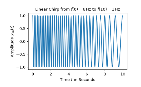
For the first example, a linear chirp ranging from 6 Hz to 1 Hz over 10 seconds is plotted:
>>> import numpy as np
>>> from matplotlib.pyplot import tight_layout
>>> from scipy.signal import chirp, square, ShortTimeFFT
>>> from scipy.signal.windows import gaussian
>>> import matplotlib.pyplot as plt
...
>>> N, T = 1000, 0.01  # number of samples and sampling interval for 10 s signal
>>> t = np.arange(N) * T  # timestamps
...
>>> x_lin = chirp(t, f0=6, f1=1, t1=10, method='linear')
...
>>> fg0, ax0 = plt.subplots()
>>> ax0.set_title(r"Linear Chirp from $f(0)=6\,$Hz to $f(10)=1\,$Hz")
>>> ax0.set(xlabel="Time $t$ in Seconds", ylabel=r"Amplitude $x_\text{lin}(t)$")
>>> ax0.plot(t, x_lin)
>>> plt.show()
The following four plots each show the short-time Fourier transform of a chirp ranging from 45 Hz to 5 Hz with different values for the parameter method (and vertex_zero):
>>> x_qu0 = chirp(t, f0=45, f1=5, t1=N*T, method='quadratic', vertex_zero=True)
>>> x_qu1 = chirp(t, f0=45, f1=5, t1=N*T, method='quadratic', vertex_zero=False)
>>> x_log = chirp(t, f0=45, f1=5, t1=N*T, method='logarithmic')
>>> x_hyp = chirp(t, f0=45, f1=5, t1=N*T, method='hyperbolic')
...
>>> win = gaussian(50, std=12, sym=True)
>>> SFT = ShortTimeFFT(win, hop=2, fs=1/T, mfft=800, scale_to='magnitude')
>>> ts = ("'quadratic', vertex_zero=True", "'quadratic', vertex_zero=False",
...       "'logarithmic'", "'hyperbolic'")
>>> fg1, ax1s = plt.subplots(2, 2, sharex='all', sharey='all',
...                          figsize=(6, 5),  layout="constrained")
>>> for x_, ax_, t_ in zip([x_qu0, x_qu1, x_log, x_hyp], ax1s.ravel(), ts):
...     aSx = abs(SFT.stft(x_))
...     im_ = ax_.imshow(aSx, origin='lower', aspect='auto', extent=SFT.extent(N),
...                      cmap='plasma')
...     ax_.set_title(t_)
...     if t_ == "'hyperbolic'":
...         fg1.colorbar(im_, ax=ax1s, label='Magnitude $|S_z(t,f)|$')
>>> _ = fg1.supxlabel("Time $t$ in Seconds")  # `_ =` is needed to pass doctests
>>> _ = fg1.supylabel("Frequency $f$ in Hertz")
>>> plt.show()
Finally, the short-time Fourier transform of a complex-valued linear chirp ranging from -30 Hz to 30 Hz is depicted:
>>> z_lin = chirp(t, f0=-30, f1=30, t1=N*T, method="linear", complex=True)
>>> SFT.fft_mode = 'centered'  # needed to work with complex signals
>>> aSz = abs(SFT.stft(z_lin))
...
>>> fg2, ax2 = plt.subplots()
>>> ax2.set_title(r"Linear Chirp from $-30\,$Hz to $30\,$Hz")
>>> ax2.set(xlabel="Time $t$ in Seconds", ylabel="Frequency $f$ in Hertz")
>>> im2 = ax2.imshow(aSz, origin='lower', aspect='auto',
...                  extent=SFT.extent(N), cmap='viridis')
>>> fg2.colorbar(im2, label='Magnitude $|S_z(t,f)|$')
>>> plt.show()
Note that using negative frequencies makes only sense with complex-valued signals. Furthermore, the magnitude of the complex exponential function is one whereas the magnitude of the real-valued cosine function is only 1/2.