scipy.optimize.

rosen#

scipy.optimize.rosen(x)[source]#

The Rosenbrock function.

The function computed is:

sum(100.0*(x[1:] - x[:-1]**2.0)**2.0 + (1 - x[:-1])**2.0)

Parameters:

xarray_like: 1-D array of points at which the Rosenbrock function is to be computed.

Returns:

ffloat: The value of the Rosenbrock function.

See also

rosen_der, rosen_hess, rosen_hess_prod

Notes

rosen has experimental support for Python Array API Standard compatible backends in addition to NumPy. Please consider testing these features by setting an environment variable SCIPY_ARRAY_API=1 and providing CuPy, PyTorch, JAX, or Dask arrays as array arguments. The following combinations of backend and device (or other capability) are supported.

Library	CPU	GPU
NumPy	✓	n/a
CuPy	n/a	✓
PyTorch	✓	✓
JAX	✓	✓
Dask	✓	✓

See Support for the array API standard for more information.

Examples

>>> import numpy as np
>>> from scipy.optimize import rosen
>>> X = 0.1 * np.arange(10)
>>> rosen(X)
76.56

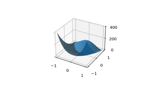
For higher-dimensional input rosen broadcasts. In the following example, we use this to plot a 2D landscape. Note that rosen_hess does not broadcast in this manner.

>>> import matplotlib.pyplot as plt
>>> from mpl_toolkits.mplot3d import Axes3D
>>> x = np.linspace(-1, 1, 50)
>>> X, Y = np.meshgrid(x, x)
>>> ax = plt.subplot(111, projection='3d')
>>> ax.plot_surface(X, Y, rosen([X, Y]))
>>> plt.show()

../../_images/scipy-optimize-rosen-1.png