scipy.integrate.

DOP853

class scipy.integrate.DOP853(fun, t0, y0, t_bound, max_step=inf, rtol=0.001, atol=1e-06, vectorized=False, first_step=None, **extraneous)

Explicit Runge-Kutta method of order 8.

This is a Python implementation of “DOP853” algorithm originally written in Fortran [1], [2]. Note that this is not a literal translation, but the algorithmic core and coefficients are the same.

Can be applied in the complex domain.

Parameters:

funcallable

Right-hand side of the system. The calling signature is fun(t, y). Here, t is a scalar, and there are two options for the ndarray y: It can either have shape (n,); then fun must return array_like with shape (n,). Alternatively it can have shape (n, k); then fun must return an array_like with shape (n, k), i.e. each column corresponds to a single column in y. The choice between the two options is determined by vectorized argument (see below).

t0float

Initial time.

y0array_like, shape (n,)

Initial state.

t_boundfloat

Boundary time - the integration won’t continue beyond it. It also determines the direction of the integration.

max_stepfloat, optional

Maximum allowed step size. Default is np.inf, i.e. the step size is not bounded and determined solely by the solver.

rtol, atolfloat and array_like, optional

Relative and absolute tolerances. The solver keeps the local error estimates less than atol + rtol * abs(y). Here rtol controls a relative accuracy (number of correct digits), while atol controls absolute accuracy (number of correct decimal places). To achieve the desired rtol, set atol to be smaller than the smallest value that can be expected from rtol * abs(y) so that rtol dominates the allowable error. If atol is larger than rtol * abs(y) the number of correct digits is not guaranteed. Conversely, to achieve the desired atol set rtol such that rtol * abs(y) is always smaller than atol. If components of y have different scales, it might be beneficial to set different atol values for different components by passing array_like with shape (n,) for atol. Default values are 1e-3 for rtol and 1e-6 for atol.

vectorizedbool, optional

Whether fun is implemented in a vectorized fashion. Default is False.

first_stepfloat or None, optional

Initial step size. Default is None which means that the algorithm should choose.

**extraneous

Any additional keyword arguments will be ignored.

Attributes:

nint

Number of equations.

statusstr

Current status of the solver: ‘running’, ‘finished’ or ‘failed’.

t_boundfloat

Boundary time.

directionfloat

Integration direction: +1 or -1.

tfloat

Current time.

yndarray

Current state.

t_oldfloat

Previous time. None if no steps were made yet.

step_sizefloat

Size of the last successful step. None if no steps were made yet.

nfevint

Number evaluations of the system’s right-hand side.

njevint

Number of evaluations of the Jacobian. Is always 0 for this solver as it does not use the Jacobian.

nluint

Number of LU decompositions. Is always 0 for this solver.

Methods

dense_output()	Compute a local interpolant over the last successful step.
step()	Perform one integration step.

References

[1]

E. Hairer, S. P. Norsett G. Wanner, “Solving Ordinary Differential Equations I: Nonstiff Problems”, Sec. II.

[2]

Page with original Fortran code of DOP853.

[3]

“Cowell’s method”, Wikipedia https://en.wikipedia.org/wiki/Orbit_modeling#Cowell’s_method

Examples

Try it in your browser!

Compute one orbit of a satellite around Earth using Cowell’s method for orbit simulations.

>>> import numpy as np
>>> import scipy.integrate as itg
>>> import matplotlib.pyplot as plt

Import the Newtonian constant of gravitation and create variables for earth’s mass and radius, and the satellite’s mass and altitude in kilograms and meters. Calculate the satellite’s orbital velocity.

>>> from scipy.constants import G
>>> mass_e, radius_e = 5.9722E24, 6.371E6
>>> mass_s, alt_s = 6E3, 2E6
>>> v_orbit = np.sqrt((G*mass_e)/(radius_e+alt_s))

Cowell’s equations for simulating two interacting bodies are a system of second-order ODEs

\[\begin{split}\begin{align*} \ddot{r}_1 &=\frac{Gm_2(r_2-r_1)}{d^3}\\ \ddot{r}_2 &= \frac{Gm_1(r_1-r_2)}{d^3} \end{align*}\end{split}\]

where \(r_1\) and \(r_2\) are the position vectors of the centers of the two bodies, \(G\) is the Newtonian constant of gravitation, and \(m_1\) and \(m_2\) are the masses of the two bodies. The distance between the centers of the two bodies is \(d = \lVert r_1 - r_2 \rVert\).

To convert Cowell’s equations into a system of first-order ODEs, introduce variables \(k_1\) and \(k_2\) for the velocity of each body.

\[\begin{split}\begin{align*} \dot{r}_1 &= k_1\\ \dot{r}_2 &= k_2\\ \dot{k}_1 &=\frac{Gm_2(r_2-r_1)}{d^3}\\ \dot{k}_2 &=\frac{Gm_1(r_1-r_2)}{d^3} \end{align*}\end{split}\]

Then, define a function that returns the right-hand side of the expanded system.

>>> def cowell(t, r):
...    # location and velocity vectors
...    r1, k1, r2, k2 = r.reshape(4,3)
...    # system coefficient
...    dist = r2 - r1
...    coeff = (G*dist/(np.linalg.norm(dist)**3))
...    # system equations
...    return np.concatenate([k1, coeff*mass_s, k2, -coeff*mass_e])

cowell accepts a vector containing the coordinates for first body’s position and velocity followed by the coordinates for the second body’s position and velocity.

Set the Earth’s initial position and velocity to zero. Set the satellite’s initial position to be the sum of the Earth’s radius and the satellite’s altitude on the x-axis, and its initial velocity to be its orbital velocity in the y-direction. Combine the initial conditions for both bodies in an initial conditions vector.

>>> init_e = np.zeros(6)
>>> init_s = [radius_e + alt_s, 0, 0, 0, v_orbit, 0]
>>> inits = np.concatenate((init_e, init_s))

Create a solver object using the initial conditions.

>>> solver = itg.DOP853(cowell, 0, inits, 1E8, max_step=50)

Use the initial state to create an array in which to store the estimated solution.

>>> solr = solver.y

Run the solver for a trial 120 integration steps, then plot earth’s trajectory in blue and the satellite’s trajectory in orange.

>>> for _ in range(120):
...     solver.step()
...     solr = np.vstack((solr, solver.y))

>>> x_e, y_e, z_e = solr.T[0:3]
>>> x_s, y_s, z_s = solr.T[6:9]

>>> fig1 = plt.figure()
>>> ax1 = fig1.add_subplot(projection='3d')
>>> ax1.plot(x_e, y_e, z_e, 'bo')
>>> ax1.plot(x_s, y_s, z_s, color='orange')
>>> ax1.set(xlabel='x', ylabel='y', zlabel='z')
>>> plt.show()

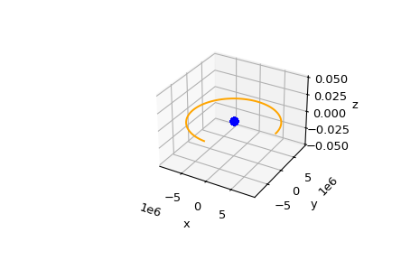
The figure shows that the Earth is approximately stationary and the satellite orbits around it. The satellite orbit has a gap.

To calculate the rest of the orbit, run the solver for another 40 integration steps.

>>> for _ in range(40):
...     solver.step()
...     solr = np.vstack((solr, solver.y))

Plot the updated solution.

>>> x_e, y_e, z_e = solr.T[0:3]
>>> x_s, y_s, z_s = solr.T[6:9]

>>> fig2 = plt.figure()
>>> ax2 = fig2.add_subplot(projection='3d')
>>> ax2.plot(x_e, y_e, z_e, 'bo')
>>> ax2.plot(x_s, y_s, z_s, color='orange')
>>> ax2.set(xlabel='x', ylabel='y', zlabel='z')
>>> plt.show()

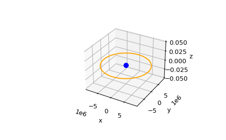
The additional 40 integration steps close the gap in the orbit.

Go BackOpen In Tab