1
2
3
4
5
6
7
8
9
10
11
12
13
14
15
16
17
18
19
20
21
22
23
24
25
26 """
27 Naive but fairly general implementation of a Kalman Filter, together with
28 some examples.
29
30
31 This program is based on the following paper:
32 Greg Welsh and Garry Bishop. An Introduction to the Kalman Filter.
33 http://www.cs.unc.edu/~welch/kalman/kalmanIntro.html
34
35 See also:
36 http://en.wikipedia.org/wiki/Kalman_filter
37
38
39 A Kalman filter is an Algorithm to estimate the states of a linear system
40 from noisy measurements. It must know the system's parameters, as well as
41 the (noisy) inputs and outputs.
42
43 A linear system can be interpreted as a system of linear differential
44 equations, in a time discete form. Therfore the state variables of many
45 physical systems can be estimated by a Kalman Filter. But there does not
46 need to be an interpretation as a differential equation. Welsh and Bishop
47 (the authors of the paper above) use the Kalman Filter to predict the
48 position of moving objects in image sequences (IMHO).
49
50 System Equations:
51 x[k] = A*x[k-1] + B*u[k] + w[k] (1)
52
53 z[k] = H*x[k] + v[k] (2)
54
55 with:
56 x: State variables (vector)
57 u: Inputs (vector)
58 z: Outputs (vector)
59
60 w,v: Random noise (vector)
61 A,B,H: Parameter matrices
62
63 (For more details of the system see the documentation of the LinSys class.)
64
65 As one can see from equation (2) it is not necessary to measure the state
66 variables directly. A Kalman Filter can estimate the system states from a
67 linear combination of them, with added noise.
68
69 Example systems:
70 - Estimate a constant value
71 - Tank with inaccurate level measurement.
72 - Spring and damper system
73
74 TODO:
75 - Optional more accurate method for simulation (scipy, Runge-Kutta)
76 Example systems:
77 - 1D Vehicle
78 """
79
80
81 from __future__ import division
82
83 import pylab
84
85 import numpy as N
86 from numpy import mat, array, c_, r_, vstack, ones, zeros, identity
87 from numpy.linalg import inv
88 from numpy.random import multivariate_normal
89
90
91
92
93
94
95 class LinSys(object):
96 """
97 General linear dynamic system. (Discrete ODE)
98
99 The class can simulate the system either step by step, or do the whole
100 simulation in one go. It stores all system parameters and it is therefore
101 used to represent the system in the Kalman filter. This class is intended
102 as a base class for more specialized simulator classes.
103
104 Random noise is generated internally, when the simulation is started. For
105 repeated computations the same random values are used.
106
107 Do not use this class to seriously solve a (continuous) differential equation.
108 The integration method used here is the very inaccurate Euler method.
109
110 System Equations:
111 Compute the state:
112 x_k = A x_{k-1} + B u_k + w_k
113
114 Compute the measurements:
115 z_k = H x_k + v_k
116
117 with:
118 x_k, x_{k-1}:
119 Current state vector, last state vector
120 u_k:
121 Control vector
122 z_k:
123 Measurement vector
124 w_k, v_k:
125 Independent random variables, with (multivariate) normal probability
126 distributions. They represent process noise and measurement noise.
127
128 w_k: Process noise: mean = 0, covariance = Q
129 v_k: Measurement noise: mean = 0, covariance = R
130
131 A, B, H:
132 Parameter matrices; system, control and measurement matrix.
133 Q, R:
134 Covariance matrices of process and measurement noise.
135
136 Usage:
137 Inherit from this class and write a problem specific __init__
138 function, that accepts arguments that are easy to understand.
139 The new __init__ must compute the matrices A, B, H, Q, R and give
140 them to LinSys.__init__.
141 For examples see: SysConstVal, SysTank, SysSpringPendulum
142
143 You can call simulate(x_0, U) to compute multiple simulation steps at
144 once:
145 >>> tank = SysTank(q=0.002, r=2) #Create system
146 >>> U = vstack((ones(10)*0.1, zeros(10))) #Create inputs
147 >>> X, Z = tank.simulate(mat('2.'), U) #Simulate
148
149 For more complex problems you can compute each simulation step
150 separately:
151 - At the beginning of the simulation call startSimulation(x_0) to supply
152 the initial values.
153 - For each time step call simulateStep(u_k). You must supply the input
154 values.
155 """
156
157 def __init__(self, A=None, B=None, H=None, Q=None, R=None, nSteps=1000):
158 """
159 Parameter:
160 A: system matrix
161 B: control input matrix
162 H: measurement matrix
163 Q: process noise covariance
164 R: measurement noise covariance
165 nSteps: number of steps for which noise will be computed
166 """
167 self.A = mat(A).copy()
168 self.B = mat(B).copy()
169 self.H = mat(H).copy()
170 self.Q = mat(Q).copy()
171 self.R = mat(R).copy()
172 self.x = mat(None)
173 self.k = None
174 self.W = None
175 self.V = None
176 self.computeNoise(nSteps)
177 self._checkMatrixCompatibility()
178
179 def _checkMatrixCompatibility(self):
180 assert self.A.shape[0] == self.A.shape[1], \
181 'Matrix "A" must be square!'
182 assert self.B.shape[0] == self.A.shape[0], \
183 'Matrix "B" must have same number of rows as matrix "A"!'
184 assert self.H.shape[1] == self.A.shape[1], \
185 'Matrix "H" must have same number of columns as matrix "A"!'
186 assert self.Q.shape[0] == self.Q.shape[1] and \
187 self.Q.shape[0] == self.A.shape[0], \
188 'Matrix "Q" must be square, ' \
189 'and it must have the same dimensions as matrix "A"'
190 assert self.R.shape[0] == self.R.shape[1]and \
191 self.R.shape[0] == self.H.shape[0], \
192 'Matrix "R" must be square, ' \
193 'and it must have the same number of rows as matrix "H"'
194
195 def computeNoise(self, nSteps):
196 """
197 Compute all process and measurement noise (self.V, self.W) in advance.
198
199 Dimensions of self.V, self.W:
200 The second dimension is the step number; so self.V[:, 2] is the
201 measurement noise for step two.
202
203 Parameter:
204 nSteps: Number of steps that should be simulated.
205 """
206 matWidth = nSteps + 1
207
208 meanW = N.zeros(self.A.shape[0])
209 W = multivariate_normal(meanW, self.Q, [matWidth])
210 self.W = mat(W).T
211
212 meanV = N.zeros(self.H.shape[0])
213 V = multivariate_normal(meanV, self.R, [matWidth])
214 self.V = mat(V).T
215
216 def _procNoise(self):
217 """Return process noise for current step."""
218 return self.W[:, self.k]
219 def _measNoise(self):
220 """Return measurement noise current step."""
221 return self.V[:, self.k]
222
223 def startSimulation(self, x_0):
224 """
225 Set initial conditions
226
227 Parameter:
228 x_0:
229 initial conditions: column vector (matrix with shape[1] == 1)
230 Return:
231 (x_0, z_k)
232 x_0:
233 state vector (initial conditions): column vector
234 (matrix with shape[1] == 1)
235 z_k:
236 first measurements: column vector (matrix with shape[1] == 1)
237 """
238 assert(self.A.shape[1] == x_0.shape[0])
239 assert(x_0.shape[1] == 1)
240
241 self.k = 0
242 self.x = mat(x_0)
243
244 z_k = self.H * self.x + self._measNoise()
245
246 return self.x, z_k
247
248 def simulateStep(self, u_k):
249 """
250 Compute one simulation step.
251
252 Parameter:
253 u_k:
254 control input: column vector (matrix with shape[1] == 1)
255 Return:
256 (x_k, z_k)
257 x_k:
258 state vector: column vector (matrix with shape[1] == 1)
259 z_k:
260 new measurements: column vector (matrix with shape[1] == 1)
261 """
262
263 x_new = self.A * self.x + self.B * u_k + self._procNoise()
264
265
266 self.k += 1
267 self.x = x_new
268
269 z_k = self.H * self.x + self._measNoise()
270
271 return self.x, z_k
272
273 def simulate(self, x_0, U, computeNoiseAgain=False):
274 """
275 Compute multiple time steps. The simulation is run until the control
276 inputs (U) are exhausted.
277
278 Dimensions of input and outputs:
279 The second dimension is the step number; so U[:,2] is the control
280 input for step three.
281
282 Parameter:
283 x_0:
284 initial conditions: 1D array or matrix. Will be converted to
285 column vector.
286 U:
287 Control inputs: 2D Array. 2nd dimension is step number.
288 computeNoiseAgain:
289 If True: compute new random noise even if it has already been
290 computed.
291 If False: compute noise only if none exists.
292 Default is False.
293 Return:
294 (X, Z)
295 X:
296 states: 2D Array; 2nd dimension is step number.
297 Z:
298 measurements: 2D Array; 2nd dimension is step number.
299 """
300
301 x_0 = mat(x_0)
302 if x_0.shape[0] == 1:
303 x_0 = x_0.T
304 assert x_0.shape[1] == 1
305 assert x_0.shape[0] == self.A.shape[1]
306
307 U = mat(U)
308 assert U.shape[0] == self.B.shape[1]
309
310 X = mat(N.zeros((x_0.shape[0], U.shape[1])))
311 Z = mat(N.zeros((self.H.shape[0], U.shape[1])))
312
313 if self.V.shape[1] < U.shape[1] or self.W.shape[1] < U.shape[1] or \
314 computeNoiseAgain:
315 self.computeNoise(U.shape[1])
316
317 dummy, z_k = self.startSimulation(x_0)
318 X[:, 0] = x_0
319 Z[:, 0] = z_k
320
321 for k in range(1, U.shape[1]):
322
323
324 x_k, z_k = self.simulateStep(U[:, k-1])
325 X[:, k] = x_k
326 Z[:, k] = z_k
327
328 return N.asarray(X), N.asarray(Z)
329
330
331 class KalmanFilter(object):
332 """
333 Kalman Filter for use together with LinSys objects.
334
335 A Kalman filter estimates the states of a linear system from noisy
336 measurements. It must know the system's parameters, and (noisy) inputs
337 and outputs. The system parameters are taken from a LinSys instance.
338 The inputs and outputs must be given at each step.
339
340 As a convenience, the function estimate(...) can process multiple
341 measurements and control inputs in one go.
342
343 Usage:
344 Create system and inputs; then simulate the system
345 >>> tank = SysTank(q=0.002, r=2) #Create system
346 >>> U = vstack((ones(10)*0.1, zeros(10))) #Create inputs
347 >>> X, Z = tank.simulate(mat('2.'), U) #Simulate
348
349 Create a Filter instance, and estimate system state from noisy measurements:
350 >>> kFilt = KalmanFilter(tank) #Create Filter
351 >>> X_hat = kFilt.estimate(Z, U) #Estimate
352
353 For complex problems each estimation step can be done separately.
354 - Start the estimation with a call to startEstimation()
355 - Compute one estimate with estimateStep(...)
356 In the loop that computes the estimation steps you will most likely also
357 compute system states (simulateStep) and control values.
358 """
359
360 def __init__(self, linearSystem=None):
361 """
362 Parameter:
363 linearSystem:
364 The linear system: LinSys.
365 """
366 self.sys = linearSystem
367 self.x_hat = mat(None)
368 self.P = mat(None)
369
370 def startEstimation(self, x_hat_0=None, P_0=None):
371 """
372 Determine start values for the the estimation algorithm.
373
374 Parameter:
375 x_hat_0:
376 Start value for estimated system states. (the algorithm can
377 guess this value).
378 P_0:
379 Start value for estimation error covariance matrix (the
380 algorithm can guess this value).
381 Return:
382 (x_hat_0, P_0)
383 """
384 xLen = self.sys.A.shape[0]
385
386 self.x_hat = mat(x_hat_0).copy() if x_hat_0 is not None else \
387 mat(N.zeros(xLen)).T
388
389 self.P = mat(P_0).copy() if P_0 is not None else \
390 mat(N.identity(xLen))
391
392 return self.x_hat, self.P
393
394 def estimateStep(self, z_k, u_k1):
395 """
396 Perform one estimation step.
397
398 Function takes new measurements and control values. From these inputs
399 it computes new estimates for the linear system's state and for the
400 estimation error covariance.
401 (System state and covariance are both returned and stored as data
402 attributes.)
403
404 This is the complete algorithm of the Kalman filter.
405
406 Parameter
407 z_k : current measurements: vector (matrix with shape[1] == 1)
408 u_k1: control values from last time step. They caused the current
409 measurements: vector (matrix with shape[1] == 1)
410
411 Return
412 (x_hat, P)
413 x_hat: new estimated state of linear system
414 P: new estimation error covariance
415 """
416
417 A = self.sys.A; B = self.sys.B; H = self.sys.H
418 Q = self.sys.Q; R = self.sys.R
419
420 I = mat(N.identity(self.x_hat.shape[0]))
421
422
423 x_old = self.x_hat
424 P_old = self.P
425
426
427
428
429
430 x_pri = A * x_old + B * u_k1
431 P_pri = A * P_old * A.T + Q
432
433
434
435 K = P_pri * H.T * inv(H * P_pri * H.T + R)
436 x_hat = x_pri + K*(z_k - H*x_pri)
437 P = (I - K*H) * P_pri
438
439
440 self.x_hat = x_hat
441 self.P = P
442
443 return x_hat, P
444
445 def estimate(self, Z, U, x_hat_0=None, P_0=None):
446 """
447 Estimate multiple time steps. The algorithm is run until the
448 measurements (Z) and control inputs (U) are exhausted.
449
450 Dimensions of input and outputs:
451 The second dimension is the step number; so U[:, 2] is the control
452 input for step two.
453
454 Parameter:
455 Z:
456 Measured values: 2D Array. 2nd dimension is step number.
457 U:
458 Control inputs to the linear system: 2D Array.
459 2nd dimension is step number.
460 x_hat_0:
461 Start value for estimated system states.(If None: algorithm
462 will guess this value).
463 P_0:
464 Start value for estimation error covariance matrix (If None:
465 algorithm will guess this value).
466 Return:
467 X_hat:
468 Estimated state variables of the linear system.
469 2D Array. First dimension is step number.
470 """
471
472 Z = mat(Z)
473 assert Z.shape[0] == self.sys.H.shape[0], \
474 'Parameter Z: 2nd dimension must be %d' % self.sys.H.shape[0]
475 U = mat(U)
476 assert U.shape[0] == self.sys.B.shape[1], \
477 'Parameter U: 2nd dimension must be %d' % self.sys.B.shape[1]
478 assert Z.shape[1] == U.shape[1], \
479 'Parameters Z, U: Arrays must contain data for same number of steps.'
480
481
482 X_hat = mat(zeros((self.sys.A.shape[0], Z.shape[1])))
483
484 X_hat[:, 0], dummy = self.startEstimation(x_hat_0=x_hat_0, P_0=P_0)
485 for k in range(1, Z.shape[1]):
486
487
488 x_hat_k, P_k = self.estimateStep(Z[:,k], U[:,k-1])
489 X_hat[:, k] = x_hat_k
490
491
492 return N.asarray(X_hat)
493
494
495 class PidController(object):
496 """Simple PID controller"""
497 def __init__(self, kp, ki, kd, ts=1.):
498 """
499 Parameter:
500 kp:
501 Proportional Gain
502 ki:
503 Integral Gain
504 kd:
505 Derivative Gain
506 ts:
507 Time step; default = 1
508 """
509 self.kp = float(kp)
510 self.ki = float(ki)
511 self.kd = float(kd)
512 self.ts = float(ts)
513 self.errInt = 0.
514 self.errOld = 0.
515
516 def computeStep(self, error):
517 """
518 Compute one new control value.
519
520 - Parameter
521 error:
522 Current error: float
523 - Return
524 New control value: float
525 """
526
527 self.errInt += self.ts * error
528
529 dErr = (error - self.errOld)/self.ts
530 self.errOld = error
531
532 return self.kp * error + self.ki * self.errInt + self.kd * dErr
533
534
535
536
537
538
539 class SysConstVal(LinSys):
540 """
541 Very simple system where the state values remain constant.
542
543 The control inputs are ignored but they must be given.
544 u_k.shape == (1,1); or U.shape == (1,number_of_steps)
545
546 The constant values (that the Kalman filter should guess later) are
547 specified as start values (x_0) for the state vector. The methods
548 startSimulation(...) and simulate(...) both take start values.
549 """
550
551 def __init__(self, n=2, R=mat('0.1, 0; 0, 0.1')):
552 """
553 Parameter:
554 n:
555 Number of constant values
556 R:
557 Covariance matrix of measurement noise. Must have shape (n,n)
558 """
559 assert R.shape[0] == n and R.shape[1] == n, \
560 'R must be square and must have shape (%d,%d)' % (n,n)
561
562 A = N.identity(n)
563 B = ones((n,1))
564 H = N.identity(n)
565 Q = zeros((n,n))
566 LinSys.__init__(self, A, B, H, Q, R)
567
568
569 class SysTank(LinSys):
570 """
571 Tank with inlet valve and outlet valve.
572
573 u[0] is inlet, u[1] is outlet
574
575 Sketch::
576 -----
577 u[0] --> ~~~~~~.
578 ----- ~
579 || ~ ||
580 ||~~~~~~~~||......................
581 ||~~~~~~~~|| ^
582 ||~~~~~~~~||---- | x
583 ||~~~~~~~~~~~~~~ --> u[1] v
584 ||=========-----..................
585
586 Difference Equation:
587 x_k = x_{k-1} + ts * u[0] - ts * u[1] + w_k
588 Noisy measurement:
589 z_k = x_k + v_k
590 with:
591 ts : temporal step size
592 w_k, v_k : noise
593 """
594
595 def __init__(self, ts=1., q=0.001, r=0.5):
596 """
597 Parameter:
598 ts:
599 Time between steps.
600 q:
601 Variance of process noise: float
602 r:
603 Variance of measurement noise: float
604 """
605 A = mat('1.')
606 B = mat([[ts, -ts]])
607 H = mat('1.')
608 Q = mat(float(q))
609 R = mat(float(r))
610 LinSys.__init__(self, A, B, H, Q, R)
611
612
613 class SysSpringPendulum(LinSys):
614 """
615 One dimensional spring pendulum with damper.
616
617 Sketch::
618 x, v, a
619 :--------->
620 || :
621 || c1 +------+
622 ||/\/\/\/\/| |
623 || d1 | |
624 || |----- | m | vibrating mass
625 ||=| ]===| |
626 || |----- | |---> F_i forces
627 || +------+
628 ||
629
630 Differential equations:
631 sum(F_i) = m*a = -c1 * x - d1 * v + F_load + F_control
632 a = diff(v,t)
633 v = diff(x, t)
634
635 Difference equations:
636 v_k = v_{k-1} - c1*ts/m * x_k - d1*ts/m * v_k
637 + ts/m * F_load + ts/m * F_control + noiseP1_k
638 x_k = x_{k-1} + ts * v_k + noiseP2_k
639
640 with:
641 ts : time step size (delta t)
642 noiseP1_k, noiseP2_k : process noise
643
644 Measurement model:
645 z1_k = x_k + noiseM2_k - you can only measure the position
646
647 state vector: x = mat([[v_k], [x_k]])
648 (control) input vector: u = mat([[F_load], [F_control]])
649 """
650
651 def __init__(self, m=1., c1=0.04, d1=0.1, ts=1., q=0.001, r=0.1):
652 """
653 Parameter:
654 m: Mass : float
655 c1: Spring constant : float
656 d1: Damping constant : float
657 ts: Time between steps. : float
658 q: Variance of process noise. : float
659 r: Variance of measurement noise. : float
660 """
661
662 omega = N.sqrt(c1/m)
663 period = 2 * N.pi / omega
664 damping = d1/N.sqrt(c1*m)
665 dStrong = 'yes' if damping > 1 else 'no'
666 print 'Period (T): %g. Circular frequency: %g.' % (period, omega)
667 print 'Damping: %g; strong damping? %s' % (damping, dStrong)
668
669 A = mat([[1.-d1*ts/m, -c1*ts/m],
670 [ts, 1. ]])
671 B = mat([[ts/m, ts/m],
672 [0., 0. ]])
673 H = mat([[0., 1.]])
674
675 Q = mat([[q, 0. ],
676 [0., q/100]])
677 R = mat([[r]])
678
679 LinSys.__init__(self, A, B, H, Q, R)
680
681
682
683
684
685
686 if __name__ == '__main__':
687
688
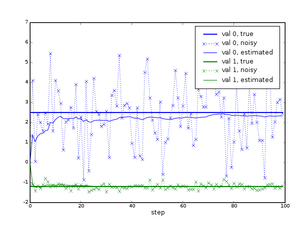
689 def experiment_ConstantValue():
690
691
692
693 constSys = SysConstVal(n=2, R=mat('2., 0; 0, 0.02'))
694 U=N.zeros((1, 100))
695 X, Z = constSys.simulate(x_0=mat('2.5; -1.2'), U=U)
696
697
698 kFilt = KalmanFilter(constSys)
699 X_hat = kFilt.estimate(Z, U)
700
701
702 pylab.figure()
703
704 pylab.plot(X[0], 'b-', label='val 0, true', linewidth=2)
705 pylab.plot(Z[0], 'b:x', label='val 0, noisy', linewidth=1)
706 pylab.plot(X_hat[0], 'b-', label='val 0, estimated', linewidth=1)
707
708 pylab.plot(X[1], 'g-', label='val 1, true', linewidth=2)
709 pylab.plot(Z[1], 'g:x', label='val 1, noisy', linewidth=1)
710 pylab.plot(X_hat[1], 'g-', label='val 1, estimated', linewidth=1)
711
712 pylab.xlabel('step')
713 pylab.legend()
714 pylab.savefig('kalman_filter_constantValue.png', dpi=75)
715 experiment_ConstantValue()
716
717
718
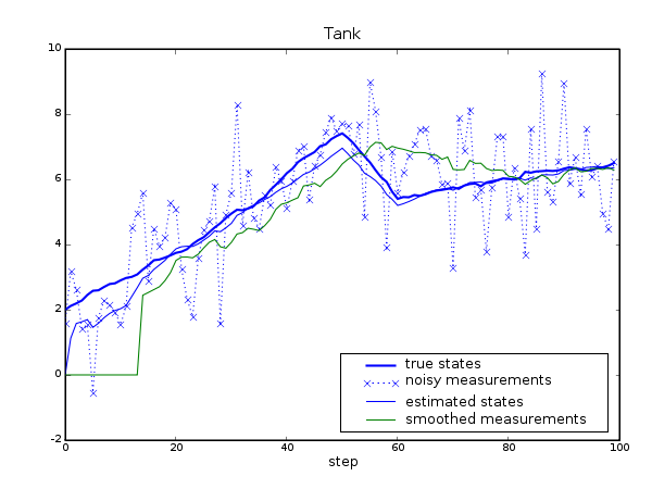
719 def experiment_tank():
720
721 valveIn = ones(100)*0.1
722 valveOut = r_[zeros(50), ones(10)*0.3, ones(40)*0.08]
723 U = vstack((valveIn, valveOut))
724
725 tank = SysTank(q=0.002, r=2)
726 X, Z = tank.simulate(x_0=mat('2.'), U=U)
727
728 kFilt = KalmanFilter(tank)
729 X_hat = kFilt.estimate(Z, U)
730
731
732 kernelSize = 15
733 kernel = ones(kernelSize) / kernelSize
734 Z_smooth = N.zeros_like(Z.ravel())
735 Z_smooth[kernelSize-1:] = N.correlate(Z.ravel(), kernel, 'valid')
736
737
738 pylab.figure()
739 pylab.plot(X[0], 'b-', label='true states', linewidth=2)
740 pylab.plot(Z[0], 'b:x', label='noisy measurements', linewidth=1)
741 pylab.plot(X_hat[0], 'b-', label='estimated states', linewidth=1)
742 pylab.plot(Z_smooth, 'g-', label='smoothed measurements', linewidth=1)
743 pylab.xlabel('step')
744 pylab.legend(loc='lower right')
745 pylab.title('Tank')
746 pylab.savefig('kalman_filter_tank.png', dpi=75)
747 experiment_tank()
748
749
750
751 def experiment_SpringPendulum():
752
753 def plotFigure(X, X_hat, Z, U, SetPoint=None,
754 title='Spring Pendulum', legendLoc='upper left'):
755 X = N.asarray(X); X_hat = N.asarray(X_hat); Z = N.asarray(Z)
756 U = N.asarray(U);
757 pylab.figure()
758 if SetPoint is not None:
759 SetPoint = N.asarray(SetPoint)
760 pylab.plot(SetPoint[0],'y-', label='set-point', linewidth=1)
761
762 pylab.plot(U[0], 'r-', label='F load', linewidth=1)
763 pylab.plot(U[1], 'm-', label='F control', linewidth=1)
764
765 pylab.plot(X[0], 'g-', label='v true', linewidth=2)
766 pylab.plot(X_hat[0], 'g-', label='v estimated', linewidth=1)
767 pylab.plot(X[1], 'b-', label='x true', linewidth=2)
768 pylab.plot(Z[0], 'b:x', label='x measured', linewidth=1)
769 pylab.plot(X_hat[1], 'b-', label='x estimated', linewidth=1)
770 pylab.xlabel('step')
771 pylab.legend(loc=legendLoc)
772 pylab.title(title)
773
774 ts = 0.5
775 nSteps = 200
776
777
778
779
780
781
782
783
784 pendu = SysSpringPendulum(m=1., c1=0.04, d1=0.1, ts=ts, q=0.004, r=2.)
785 kFilt = KalmanFilter(pendu)
786
787
788 def onlyNoise():
789
790 U = zeros((2, nSteps))
791
792 X, Z = pendu.simulate(x_0=mat('0.; 0.'), U=U)
793
794
795 X_hat = kFilt.estimate(Z, U)
796 plotFigure(X, X_hat, Z, U,
797 title='Spring Pendulum - Only Noise')
798 pylab.savefig('kalman_filter_springPendulum_onlyNoise.png', dpi=75)
799
800
801
802 def impulseExcitation():
803
804
805 U = zeros((2, nSteps))
806 U[0, int(nSteps/2)] = 2.5/ts
807
808 X, Z = pendu.simulate(x_0=mat('0.; 0.'), U=U)
809
810
811 X_hat = kFilt.estimate(Z, U)
812 plotFigure(X, X_hat, Z, U,
813 title='Spring Pendulum - Impulse Excitation')
814 pylab.savefig('kalman_filter_springPendulum_impulseExcitation.png', dpi=75)
815 impulseExcitation()
816
817
818
819 def impulseExcitation_KalmanNotSeeForce():
820
821
822 U = zeros((2, nSteps))
823 U[0, int(nSteps/2)] = 2.5/ts
824
825 X, Z = pendu.simulate(x_0=mat('0.; 0.'), U=U)
826
827
828
829 Uzero = N.zeros_like(U)
830 X_hat = kFilt.estimate(Z, Uzero)
831 plotFigure(X, X_hat, Z, U,
832 title='Spring Pendulum - Kalman filter can not see force')
833 pylab.savefig('kalman_filter_springPendulum_KalmanNotSeeForce.png', dpi=75)
834 impulseExcitation_KalmanNotSeeForce()
835
836
837 def springPendulumController():
838
839 SetPoint = mat(zeros(nSteps))
840 SetPoint[0, int(nSteps/2):] = 8.
841
842 controllerPos = PidController(kp=0.3, ki=0.01, kd=0.0, ts=ts)
843
844 controllerDamp = PidController(kp=1.0, ki=0.0, kd=0.1, ts=ts)
845
846 X = mat(zeros((2,nSteps)))
847 X_hat = mat(zeros((2,nSteps)))
848 Z = mat(zeros((1,nSteps)))
849 U = mat(zeros((2,nSteps)))
850
851 x_k, z_k = pendu.startSimulation(x_0=mat('0.; 0.'))
852 x_hat_k, P = kFilt.startEstimation()
853 u_k = mat('0.; 0.')
854
855 for k in range(0, nSteps):
856 X[:, k] = x_k
857 Z[:, k] = z_k
858 X_hat[:, k] = x_hat_k
859 U[:, k] = u_k
860
861
862
863 pos, speed = X_hat[1, k], X_hat[0, k]
864 sp = SetPoint[0, k]
865 f_control_k = controllerPos.computeStep(sp-pos) + \
866 controllerDamp.computeStep(-speed)
867
868 u_k = mat([[0.], [f_control_k]])
869
870 x_k, z_k = pendu.simulateStep(u_k)
871 x_hat_k, P = kFilt.estimateStep(z_k, u_k)
872
873 plotFigure(X, X_hat, Z, U, SetPoint,
874 title='Spring Pendulum - Controller for position and damping')
875 pylab.savefig('kalman_filter_springPendulum_springPendulumController.png', dpi=75)
876 springPendulumController()
877
878 experiment_SpringPendulum()
879
880
881 pylab.show()