1 #! /usr/bin/env python
   2 # -*- coding: utf-8 -*-
   3 
   4 """
   5 http://www.scipy.org/Cookbook/Least_Squares_Circle
   6 """
   7 
   8 from numpy import *
   9 
  10 # Coordinates of the 2D points
  11 
  12 x = r_[  9, 35, -13,  10,  23,   0]
  13 y = r_[ 34, 10,   6, -14,  27, -10]
  14 basename = 'circle'
  15 
  16 # x = r_[36, 36, 19, 18, 33, 26]
  17 # y = r_[14, 10, 28, 31, 18, 26]
  18 # basename = 'arc'
  19 
  20 # # Code to generate random data points
  21 # R0 = 25
  22 # nb_pts = 40
  23 # dR = 1
  24 # angle =10*pi/5
  25 # theta0 = random.uniform(0, angle, size=nb_pts)
  26 # x = (10 + R0*cos(theta0) + dR*random.normal(size=nb_pts)).round()
  27 # y = (10 + R0*sin(theta0) + dR*random.normal(size=nb_pts)).round()
  28 
  29 
  30 # == METHOD 1 ==
  31 method_1 = 'algebraic'
  32 
  33 # coordinates of the barycenter
  34 x_m = mean(x)
  35 y_m = mean(y)
  36 
  37 # calculation of the reduced coordinates
  38 u = x - x_m
  39 v = y - y_m
  40 
  41 # linear system defining the center in reduced coordinates (uc, vc):
  42 #    Suu * uc +  Suv * vc = (Suuu + Suvv)/2
  43 #    Suv * uc +  Svv * vc = (Suuv + Svvv)/2
  44 Suv  = sum(u*v)
  45 Suu  = sum(u**2)
  46 Svv  = sum(v**2)
  47 Suuv = sum(u**2 * v)
  48 Suvv = sum(u * v**2)
  49 Suuu = sum(u**3)
  50 Svvv = sum(v**3)
  51 
  52 # Solving the linear system
  53 A = array([ [ Suu, Suv ], [Suv, Svv]])
  54 B = array([ Suuu + Suvv, Svvv + Suuv ])/2.0
  55 uc, vc = linalg.solve(A, B)
  56 
  57 xc_1 = x_m + uc
  58 yc_1 = y_m + vc
  59 
  60 # Calculation of all distances from the center (xc_1, yc_1)
  61 Ri_1      = sqrt((x-xc_1)**2 + (y-yc_1)**2)
  62 R_1       = mean(Ri_1)
  63 residu_1  = sum((Ri_1-R_1)**2)
  64 residu2_1 = sum((Ri_1**2-R_1**2)**2)
  65 
  66 # Decorator to count functions calls
  67 import functools
  68 def countcalls(fn):
  69     "decorator function count function calls "
  70 
  71     @functools.wraps(fn)
  72     def wrapped(*args):
  73         wrapped.ncalls +=1
  74         return fn(*args)
  75 
  76     wrapped.ncalls = 0
  77     return wrapped
  78 
  79 #  == METHOD 2 ==
  80 # Basic usage of optimize.leastsq
  81 from scipy      import optimize
  82 
  83 method_2  = "leastsq"
  84 
  85 def calc_R(xc, yc):
  86     """ calculate the distance of each 2D points from the center (xc, yc) """
  87     return sqrt((x-xc)**2 + (y-yc)**2)
  88 
  89 @countcalls
  90 def f_2(c):
  91     """ calculate the algebraic distance between the 2D points and the mean circle centered at c=(xc, yc) """
  92     Ri = calc_R(*c)
  93     return Ri - Ri.mean()
  94 
  95 center_estimate = x_m, y_m
  96 center_2, ier = optimize.leastsq(f_2, center_estimate)
  97 
  98 xc_2, yc_2 = center_2
  99 Ri_2       = calc_R(xc_2, yc_2)
 100 R_2        = Ri_2.mean()
 101 residu_2   = sum((Ri_2 - R_2)**2)
 102 residu2_2  = sum((Ri_2**2-R_2**2)**2)
 103 ncalls_2   = f_2.ncalls
 104 
 105 # == METHOD 2b ==
 106 # Advanced usage, with jacobian
 107 method_2b  = "leastsq with jacobian"
 108 
 109 def calc_R(xc, yc):
 110     """ calculate the distance of each 2D points from the center c=(xc, yc) """
 111     return sqrt((x-xc)**2 + (y-yc)**2)
 112 
 113 @countcalls
 114 def f_2b(c):
 115     """ calculate the algebraic distance between the 2D points and the mean circle centered at c=(xc, yc) """
 116     Ri = calc_R(*c)
 117     return Ri - Ri.mean()
 118 
 119 @countcalls
 120 def Df_2b(c):
 121     """ Jacobian of f_2b
 122     The axis corresponding to derivatives must be coherent with the col_deriv option of leastsq"""
 123     xc, yc     = c
 124     df2b_dc    = empty((len(c), x.size))
 125 
 126     Ri = calc_R(xc, yc)
 127     df2b_dc[ 0] = (xc - x)/Ri                   # dR/dxc
 128     df2b_dc[ 1] = (yc - y)/Ri                   # dR/dyc
 129     df2b_dc       = df2b_dc - df2b_dc.mean(axis=1)[:, newaxis]
 130 
 131     return df2b_dc
 132 
 133 center_estimate = x_m, y_m
 134 center_2b, ier = optimize.leastsq(f_2b, center_estimate, Dfun=Df_2b, col_deriv=True)
 135 
 136 xc_2b, yc_2b = center_2b
 137 Ri_2b        = calc_R(xc_2b, yc_2b)
 138 R_2b         = Ri_2b.mean()
 139 residu_2b    = sum((Ri_2b - R_2b)**2)
 140 residu2_2b   = sum((Ri_2b**2-R_2b**2)**2)
 141 ncalls_2b    = f_2b.ncalls
 142 
 143 print """
 144 Method 2b :
 145 print "Functions calls : f_2b=%d Df_2b=%d""" % ( f_2b.ncalls, Df_2b.ncalls)
 146 
 147 # == METHOD 3 ==
 148 # Basic usage of odr with an implicit function definition
 149 from scipy      import  odr
 150 
 151 method_3  = "odr"
 152 
 153 @countcalls
 154 def f_3(beta, x):
 155     """ implicit definition of the circle """
 156     return (x[0]-beta[0])**2 + (x[1]-beta[1])**2 -beta[2]**2
 157 
 158 # initial guess for parameters
 159 R_m = calc_R(x_m, y_m).mean()
 160 beta0 = [ x_m, y_m, R_m]
 161 
 162 # for implicit function :
 163 #       data.x contains both coordinates of the points
 164 #       data.y is the dimensionality of the response
 165 lsc_data   = odr.Data(row_stack([x, y]), y=1)
 166 lsc_model  = odr.Model(f_3, implicit=True)
 167 lsc_odr    = odr.ODR(lsc_data, lsc_model, beta0)
 168 lsc_out    = lsc_odr.run()
 169 
 170 xc_3, yc_3, R_3 = lsc_out.beta
 171 Ri_3       = calc_R(xc_3, yc_3)
 172 residu_3   = sum((Ri_3 - R_3)**2)
 173 residu2_3  = sum((Ri_3**2-R_3**2)**2)
 174 ncalls_3   = f_3.ncalls
 175 
 176 # == METHOD 3b ==
 177 # Advanced usage, with jacobian
 178 method_3b  = "odr with jacobian"
 179 print "\nMethod 3b : ", method_3b
 180 
 181 @countcalls
 182 def f_3b(beta, x):
 183     """ implicit definition of the circle """
 184     return (x[0]-beta[0])**2 + (x[1]-beta[1])**2 -beta[2]**2
 185 
 186 @countcalls
 187 def jacb(beta, x):
 188     """ Jacobian function with respect to the parameters beta.
 189     return df_3b/dbeta
 190     """
 191     xc, yc, r = beta
 192     xi, yi    = x
 193 
 194     df_db    = empty((beta.size, x.shape[1]))
 195     df_db[0] =  2*(xc-xi)                     # d_f/dxc
 196     df_db[1] =  2*(yc-yi)                     # d_f/dyc
 197     df_db[2] = -2*r                           # d_f/dr
 198 
 199     return df_db
 200 
 201 @countcalls
 202 def jacd(beta, x):
 203     """ Jacobian function with respect to the input x.
 204     return df_3b/dx
 205     """
 206     xc, yc, r = beta
 207     xi, yi    = x
 208 
 209     df_dx    = empty_like(x)
 210     df_dx[0] =  2*(xi-xc)                     # d_f/dxi
 211     df_dx[1] =  2*(yi-yc)                     # d_f/dyi
 212 
 213     return df_dx
 214 
 215 
 216 def calc_estimate(data):
 217     """ Return a first estimation on the parameter from the data  """
 218     xc0, yc0 = data.x.mean(axis=1)
 219     r0 = sqrt((data.x[0]-xc0)**2 +(data.x[1] -yc0)**2).mean()
 220     return xc0, yc0, r0
 221 
 222 # for implicit function :
 223 #       data.x contains both coordinates of the points
 224 #       data.y is the dimensionality of the response
 225 lsc_data  = odr.Data(row_stack([x, y]), y=1)
 226 lsc_model = odr.Model(f_3b, implicit=True, estimate=calc_estimate, fjacd=jacd, fjacb=jacb)
 227 lsc_odr   = odr.ODR(lsc_data, lsc_model)    # beta0 has been replaced by an estimate function
 228 lsc_odr.set_job(deriv=3)                    # use user derivatives function without checking
 229 lsc_odr.set_iprint(iter=1, iter_step=1)     # print details for each iteration
 230 lsc_out   = lsc_odr.run()
 231 
 232 xc_3b, yc_3b, R_3b = lsc_out.beta
 233 Ri_3b       = calc_R(xc_3b, yc_3b)
 234 residu_3b   = sum((Ri_3b - R_3b)**2)
 235 residu2_3b  = sum((Ri_3b**2-R_3b**2)**2)
 236 ncalls_3b   = f_3b.ncalls
 237 
 238 print "\nFunctions calls : f_3b=%d jacb=%d jacd=%d" % (f_3b.ncalls, jacb.ncalls, jacd.ncalls)
 239 
 240 
 241 # Summary
 242 fmt = '%-22s %10.5f %10.5f %10.5f %10d %10.6f %10.6f %10.2f'
 243 print ('\n%-22s' +' %10s'*7) % tuple('METHOD Xc Yc Rc nb_calls std(Ri) residu residu2'.split())
 244 print '-'*(22 +7*(10+1))
 245 print  fmt % (method_1 , xc_1 , yc_1 , R_1 ,        1 , Ri_1.std() , residu_1 , residu2_1 )
 246 print  fmt % (method_2 , xc_2 , yc_2 , R_2 , ncalls_2 , Ri_2.std() , residu_2 , residu2_2 )
 247 print  fmt % (method_2b, xc_2b, yc_2b, R_2b, ncalls_2b, Ri_2b.std(), residu_2b, residu2_2b)
 248 print  fmt % (method_3 , xc_3 , yc_3 , R_3 , ncalls_3 , Ri_3.std() , residu_3 , residu2_3 )
 249 print  fmt % (method_3b, xc_3b, yc_3b, R_3b, ncalls_3b, Ri_3b.std(), residu_3b, residu2_3b)
 250 
 251 # plotting functions
 252 from matplotlib                 import pyplot as p, cm, colors
 253 p.close('all')
 254 
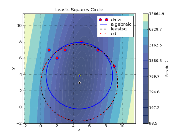
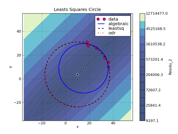
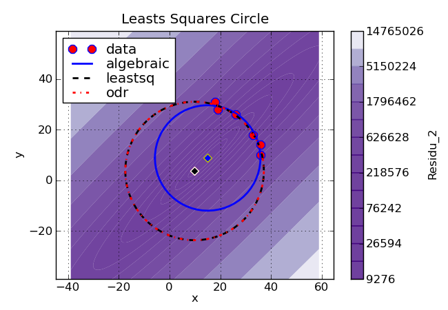
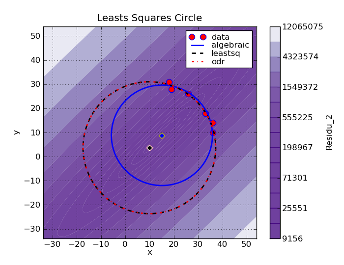
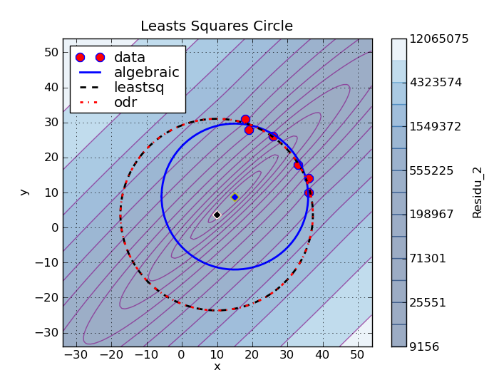
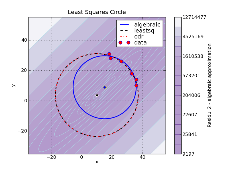
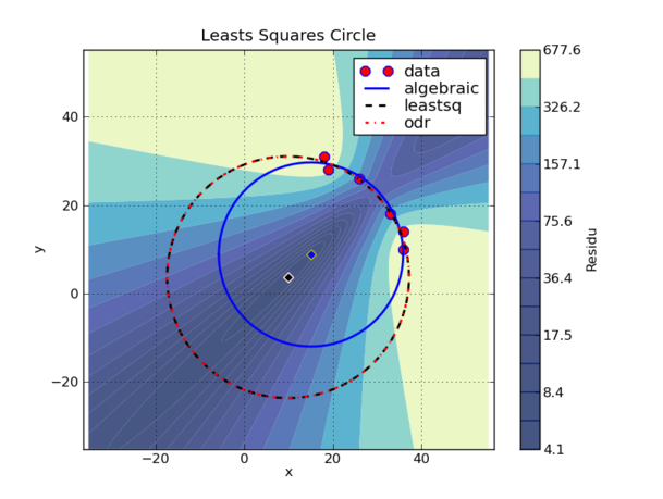
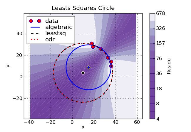
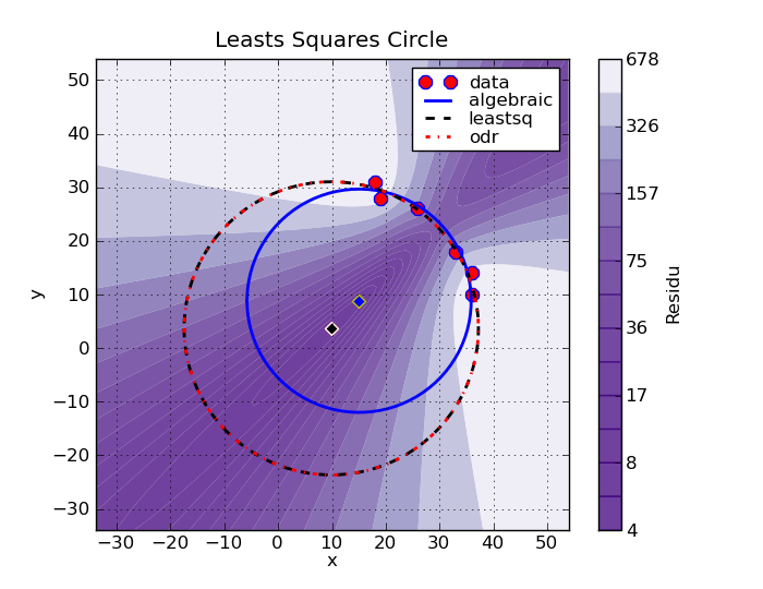
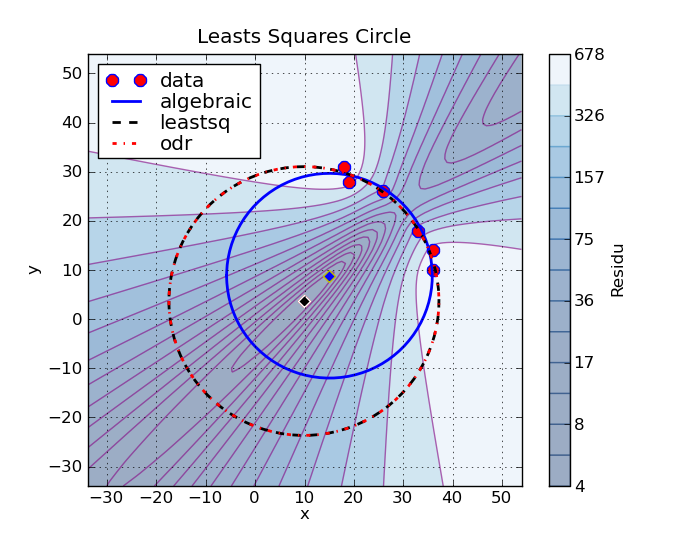
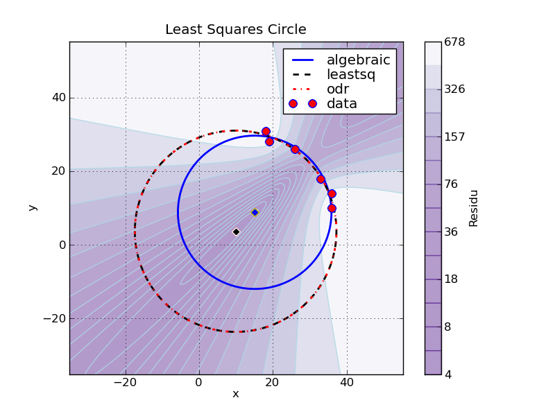
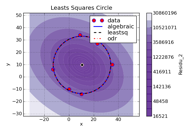
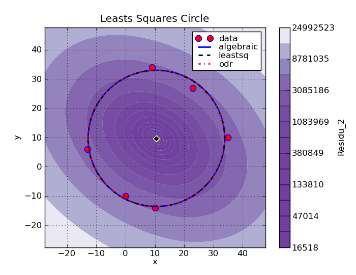
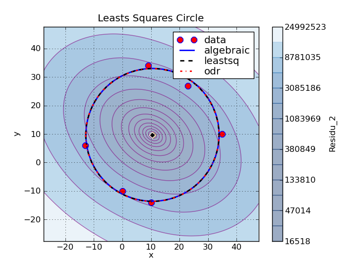
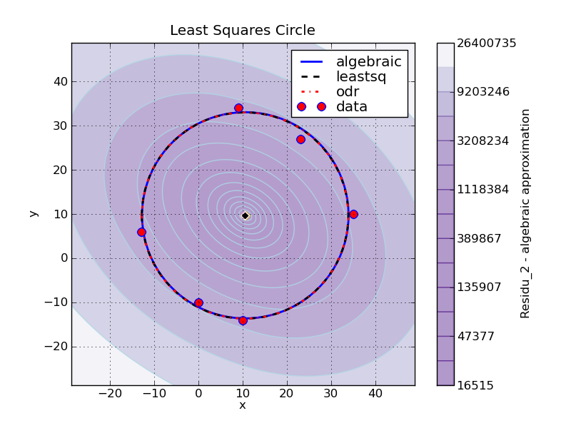
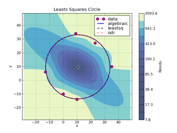
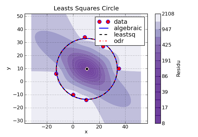
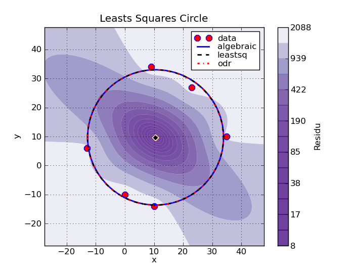
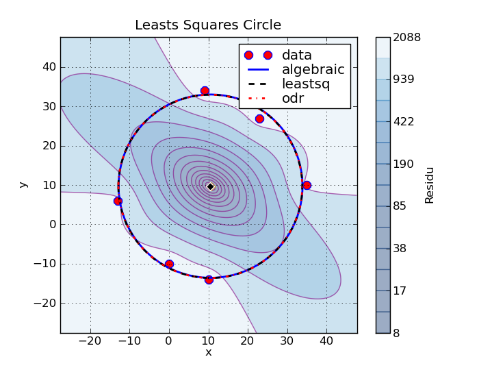
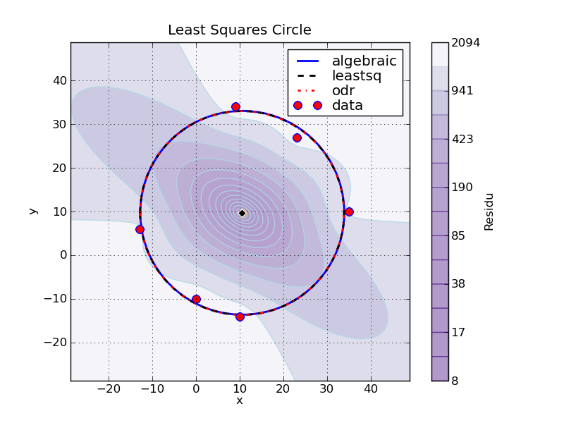
 255 def plot_all(residu2=False):
 256     """ Draw data points, best fit circles and center for the three methods,
 257     and adds the iso contours corresponding to the fiel residu or residu2
 258     """
 259 
 260     f = p.figure( facecolor='white')  #figsize=(7, 5.4), dpi=72,
 261     p.axis('equal')
 262 
 263     theta_fit = linspace(-pi, pi, 180)
 264 
 265     x_fit1 = xc_1 + R_1*cos(theta_fit)
 266     y_fit1 = yc_1 + R_1*sin(theta_fit)
 267     p.plot(x_fit1, y_fit1, 'b-' , label=method_1, lw=2)
 268 
 269     x_fit2 = xc_2 + R_2*cos(theta_fit)
 270     y_fit2 = yc_2 + R_2*sin(theta_fit)
 271     p.plot(x_fit2, y_fit2, 'k--', label=method_2, lw=2)
 272 
 273     x_fit3 = xc_3 + R_3*cos(theta_fit)
 274     y_fit3 = yc_3 + R_3*sin(theta_fit)
 275     p.plot(x_fit3, y_fit3, 'r-.', label=method_3, lw=2)
 276 
 277     p.plot([xc_1], [yc_1], 'bD', mec='y', mew=1)
 278     p.plot([xc_2], [yc_2], 'gD', mec='r', mew=1)
 279     p.plot([xc_3], [yc_3], 'kD', mec='w', mew=1)
 280 
 281     # draw
 282     p.xlabel('x')
 283     p.ylabel('y')
 284 
 285     # plot the residu fields
 286     nb_pts = 100
 287 
 288     p.draw()
 289     xmin, xmax = p.xlim()
 290     ymin, ymax = p.ylim()
 291 
 292     vmin = min(xmin, ymin)
 293     vmax = max(xmax, ymax)
 294 
 295     xg, yg = ogrid[vmin:vmax:nb_pts*1j, vmin:vmax:nb_pts*1j]
 296     xg = xg[..., newaxis]
 297     yg = yg[..., newaxis]
 298 
 299     Rig    = sqrt( (xg - x)**2 + (yg - y)**2 )
 300     Rig_m  = Rig.mean(axis=2)[..., newaxis]
 301 
 302     if residu2 : residu = sum( (Rig**2 - Rig_m**2)**2 ,axis=2)
 303     else       : residu = sum( (Rig-Rig_m)**2 ,axis=2)
 304 
 305     lvl = exp(linspace(log(residu.min()), log(residu.max()), 15))
 306 
 307     p.contourf(xg.flat, yg.flat, residu.T, lvl, alpha=0.4, cmap=cm.Purples_r) # , norm=colors.LogNorm())
 308     cbar = p.colorbar(fraction=0.175, format='%.f')
 309     p.contour (xg.flat, yg.flat, residu.T, lvl, alpha=0.8, colors="lightblue")
 310 
 311     if residu2 : cbar.set_label('Residu_2 - algebraic approximation')
 312     else       : cbar.set_label('Residu')
 313 
 314     # plot data
 315     p.plot(x, y, 'ro', label='data', ms=8, mec='b', mew=1)
 316     p.legend(loc='best',labelspacing=0.1 )
 317 
 318     p.xlim(xmin=vmin, xmax=vmax)
 319     p.ylim(ymin=vmin, ymax=vmax)
 320 
 321     p.grid()
 322     p.title('Least Squares Circle')
 323     p.savefig('%s_residu%d.png' % (basename, 2 if residu2 else 1))
 324 
 325 plot_all(residu2=False)
 326 plot_all(residu2=True )
 327 
 328 p.show()
 329 # vim: set et sts=4 sw=4: