This page shows you how to fit experimental data and plots the results using matplotlib.
Contents
Fit examples with sinusoidal functions
Generating the data
Using real data is much more fun, but, just so that you can reproduce this example I will generate data to fit
   1 from pylab import *
   2 from scipy import *
   3
   4 # if you experience problem "optimize not found", try to uncomment the following line. The problem is present at least at Ubuntu Lucid python scipy package
   5 # from scipy import optimize
   6
   7 # Generate data points with noise
   8 num_points = 150
   9 Tx = linspace(5., 8., num_points)
  10 Ty = Tx
  11
  12 tX = 11.86*cos(2*pi/0.81*Tx-1.32) + 0.64*Tx+4*((0.5-rand(num_points))*exp(2*rand(num_points)**2))
  13 tY = -32.14*cos(2*pi/0.8*Ty-1.94) + 0.15*Ty+7*((0.5-rand(num_points))*exp(2*rand(num_points)**2))
Fitting the data
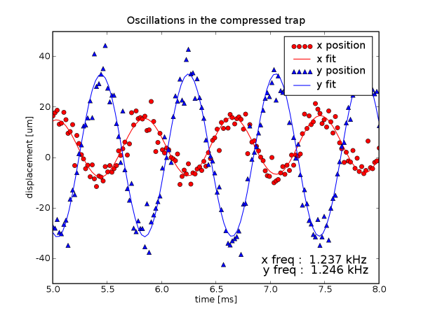
We now have two sets of data: Tx and Ty, the time series, and tX and tY, sinusoidal data with noise. We are interested in finding the frequency of the sine wave.
   1 # Fit the first set
   2 fitfunc = lambda p, x: p[0]*cos(2*pi/p[1]*x+p[2]) + p[3]*x # Target function
   3 errfunc = lambda p, x, y: fitfunc(p, x) - y # Distance to the target function
   4 p0 = [-15., 0.8, 0., -1.] # Initial guess for the parameters
   5 p1, success = optimize.leastsq(errfunc, p0[:], args=(Tx, tX))
   6
   7 time = linspace(Tx.min(), Tx.max(), 100)
   8 plot(Tx, tX, "ro", time, fitfunc(p1, time), "r-") # Plot of the data and the fit
   9
  10 # Fit the second set
  11 p0 = [-15., 0.8, 0., -1.]
  12 p2,success = optimize.leastsq(errfunc, p0[:], args=(Ty, tY))
  13
  14 time = linspace(Ty.min(), Ty.max(), 100)
  15 plot(Ty, tY, "b^", time, fitfunc(p2, time), "b-")
  16
  17 # Legend the plot
  18 title("Oscillations in the compressed trap")
  19 xlabel("time [ms]")
  20 ylabel("displacement [um]")
  21 legend(('x position', 'x fit', 'y position', 'y fit'))
  22
  23 ax = axes()
  24
  25 text(0.8, 0.07,
  26      'x freq :  %.3f kHz \n y freq :  %.3f kHz' % (1/p1[1],1/p2[1]),
  27      fontsize=16,
  28      horizontalalignment='center',
  29      verticalalignment='center',
  30      transform=ax.transAxes)
  31
  32 show()

A clever use of the cost function
Suppose that you have the same data set: two time-series of oscillating phenomena, but that you know that the frequency of the two oscillations is the same. A clever use of the cost function can allow you to fit both set of data in one fit, using the same frequency. The idea is that you return, as a "cost" array, the concatenation of the costs of your two data sets for one choice of parameters. Thus the leastsq routine is optimizing both data sets at the same time.
   1 # Target function
   2 fitfunc = lambda T, p, x: p[0]*cos(2*pi/T*x+p[1]) + p[2]*x
   3 # Initial guess for the first set's parameters
   4 p1 = r_[-15., 0., -1.]
   5 # Initial guess for the second set's parameters
   6 p2 = r_[-15., 0., -1.]
   7 # Initial guess for the common period
   8 T = 0.8
   9 # Vector of the parameters to fit, it contains all the parameters of the problem, and the period of the oscillation is not there twice !
  10 p = r_[T, p1, p2]
  11 # Cost function of the fit, compare it to the previous example.
  12 errfunc = lambda p, x1, y1, x2, y2: r_[
  13                 fitfunc(p[0], p[1:4], x1) - y1,
  14                 fitfunc(p[0], p[4:7], x2) - y2
  15             ]
  16 # This time we need to pass the two sets of data, there are thus four "args".
  17 p,success = optimize.leastsq(errfunc, p, args=(Tx, tX, Ty, tY))
  18 time = linspace(Tx.min(), Tx.max(), 100) # Plot of the first data and the fit
  19 plot(Tx, tX, "ro", time, fitfunc(p[0], p[1:4], time),"r-")
  20
  21 # Plot of the second data and the fit
  22 time = linspace(Ty.min(), Ty.max(),100)
  23 plot(Ty, tY, "b^", time, fitfunc(p[0], p[4:7], time),"b-")
  24
  25 # Legend the plot
  26 title("Oscillations in the compressed trap")
  27 xlabel("time [ms]")
  28 ylabel("displacement [um]")
  29 legend(('x position', 'x fit', 'y position', 'y fit'))
  30
  31 ax = axes()
  32
  33 text(0.8, 0.07,
  34      'x freq :  %.3f kHz' % (1/p[0]),
  35      fontsize=16,
  36      horizontalalignment='center',
  37      verticalalignment='center',
  38      transform=ax.transAxes)
  39
  40 show()
Simplifying the syntax
Especially when using fits for interactive use, the standard syntax for optimize.leastsq can get really long. Using the following script can simplify your life:
   1 from scipy import optimize
   2 from numpy import *
   3
   4 class Parameter:
   5     def __init__(self, value):
   6             self.value = value
   7
   8     def set(self, value):
   9             self.value = value
  10
  11     def __call__(self):
  12             return self.value
  13
  14 def fit(function, parameters, y, x = None):
  15     def f(params):
  16         i = 0
  17         for p in parameters:
  18             p.set(params[i])
  19             i += 1
  20         return y - function(x)
  21
  22     if x is None: x = arange(y.shape[0])
  23     p = [param() for param in parameters]
  24     optimize.leastsq(f, p)
Now fitting becomes really easy, for example fitting to a gaussian:
Fitting gaussian-shaped data
Calculating the moments of the distribution
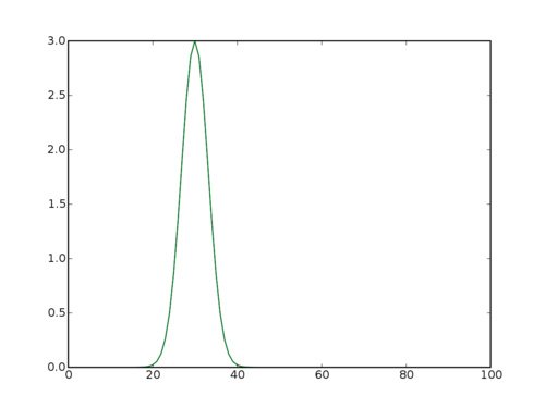
Fitting gaussian-shaped data does not require an optimization routine. Just calculating the moments of the distribution is enough, and this is much faster.
However this works only if the gaussian is not cut out too much, and if it is not too small.
   1 from pylab import *
   2
   3 gaussian = lambda x: 3*exp(-(30-x)**2/20.)
   4
   5 data = gaussian(arange(100))
   6
   7 plot(data)
   8
   9 X = arange(data.size)
  10 x = sum(X*data)/sum(data)
  11 width = sqrt(abs(sum((X-x)**2*data)/sum(data)))
  12
  13 max = data.max()
  14
  15 fit = lambda t : max*exp(-(t-x)**2/(2*width**2))
  16
  17 plot(fit(X))
  18
  19 show()

Fitting a 2D gaussian
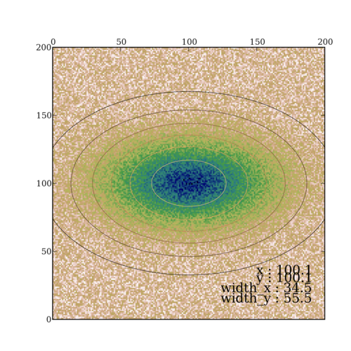
Here is robust code to fit a 2D gaussian. It calculates the moments of the data to guess the initial parameters for an optimization routine. For a more complete gaussian, one with an optional additive constant and rotation, see http://code.google.com/p/agpy/source/browse/trunk/agpy/gaussfitter.py. It also allows the specification of a known error.
   1 from numpy import *
   2 from scipy import optimize
   3
   4 def gaussian(height, center_x, center_y, width_x, width_y):
   5     """Returns a gaussian function with the given parameters"""
   6     width_x = float(width_x)
   7     width_y = float(width_y)
   8     return lambda x,y: height*exp(
   9                 -(((center_x-x)/width_x)**2+((center_y-y)/width_y)**2)/2)
  10
  11 def moments(data):
  12     """Returns (height, x, y, width_x, width_y)
  13     the gaussian parameters of a 2D distribution by calculating its
  14     moments """
  15     total = data.sum()
  16     X, Y = indices(data.shape)
  17     x = (X*data).sum()/total
  18     y = (Y*data).sum()/total
  19     col = data[:, int(y)]
  20     width_x = sqrt(abs((arange(col.size)-y)**2*col).sum()/col.sum())
  21     row = data[int(x), :]
  22     width_y = sqrt(abs((arange(row.size)-x)**2*row).sum()/row.sum())
  23     height = data.max()
  24     return height, x, y, width_x, width_y
  25
  26 def fitgaussian(data):
  27     """Returns (height, x, y, width_x, width_y)
  28     the gaussian parameters of a 2D distribution found by a fit"""
  29     params = moments(data)
  30     errorfunction = lambda p: ravel(gaussian(*p)(*indices(data.shape)) -
  31                                  data)
  32     p, success = optimize.leastsq(errorfunction, params)
  33     return p
And here is an example using it:
   1 from pylab import *
   2 # Create the gaussian data
   3 Xin, Yin = mgrid[0:201, 0:201]
   4 data = gaussian(3, 100, 100, 20, 40)(Xin, Yin) + random.random(Xin.shape)
   5
   6 matshow(data, cmap=cm.gist_earth_r)
   7
   8 params = fitgaussian(data)
   9 fit = gaussian(*params)
  10
  11 contour(fit(*indices(data.shape)), cmap=cm.copper)
  12 ax = gca()
  13 (height, x, y, width_x, width_y) = params
  14
  15 text(0.95, 0.05, """
  16 x : %.1f
  17 y : %.1f
  18 width_x : %.1f
  19 width_y : %.1f""" %(x, y, width_x, width_y),
  20         fontsize=16, horizontalalignment='right',
  21         verticalalignment='bottom', transform=ax.transAxes)
  22
  23 show()

Fitting a power-law to data with errors
Generating the data
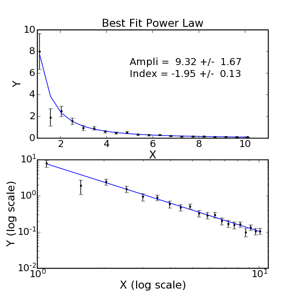
Generate some data with noise to demonstrate the fitting procedure. Data is generated with an amplitude of 10 and a power-law index of -2.0. Notice that all of our data is well-behaved when the log is taken... you may have to be more careful of this for real data.
   1 from pylab import *
   2 from scipy import *
   3
   4 # Define function for calculating a power law
   5 powerlaw = lambda x, amp, index: amp * (x**index)
   6
   7 ##########
   8 # Generate data points with noise
   9 ##########
  10 num_points = 20
  11
  12 # Note: all positive, non-zero data
  13 xdata = linspace(1.1, 10.1, num_points)
  14 ydata = powerlaw(xdata, 10.0, -2.0)     # simulated perfect data
  15 yerr = 0.2 * ydata                      # simulated errors (10%)
  16
  17 ydata += randn(num_points) * yerr       # simulated noisy data
Fitting the data
If your data is well-behaved, you can fit a power-law function by first converting to a linear equation by using the logarithm. Then use the optimize function to fit a straight line. Notice that we are weighting by positional uncertainties during the fit. Also, the best-fit parameters uncertainties are estimated from the variance-covariance matrix. You should read up on when it may not be appropriate to use this form of error estimation. If you are trying to fit a power-law distribution, this solution is more appropriate.
   1 ##########
   2 # Fitting the data -- Least Squares Method
   3 ##########
   4
   5 # Power-law fitting is best done by first converting
   6 # to a linear equation and then fitting to a straight line.
   7 #
   8 #  y = a * x^b
   9 #  log(y) = log(a) + b*log(x)
  10 #
  11
  12 logx = log10(xdata)
  13 logy = log10(ydata)
  14 logyerr = yerr / ydata
  15
  16 # define our (line) fitting function
  17 fitfunc = lambda p, x: p[0] + p[1] * x
  18 errfunc = lambda p, x, y, err: (y - fitfunc(p, x)) / err
  19
  20 pinit = [1.0, -1.0]
  21 out = optimize.leastsq(errfunc, pinit,
  22                        args=(logx, logy, logyerr), full_output=1)
  23
  24 pfinal = out[0]
  25 covar = out[1]
  26 print pfinal
  27 print covar
  28
  29 index = pfinal[1]
  30 amp = 10.0**pfinal[0]
  31
  32 indexErr = sqrt( covar[0][0] )
  33 ampErr = sqrt( covar[1][1] ) * amp
  34
  35 ##########
  36 # Plotting data
  37 ##########
  38
  39 clf()
  40 subplot(2, 1, 1)
  41 plot(xdata, powerlaw(xdata, amp, index))     # Fit
  42 errorbar(xdata, ydata, yerr=yerr, fmt='k.')  # Data
  43 text(5, 6.5, 'Ampli = %5.2f +/- %5.2f' % (amp, ampErr))
  44 text(5, 5.5, 'Index = %5.2f +/- %5.2f' % (index, indexErr))
  45 title('Best Fit Power Law')
  46 xlabel('X')
  47 ylabel('Y')
  48 xlim(1, 11)
  49
  50 subplot(2, 1, 2)
  51 loglog(xdata, powerlaw(xdata, amp, index))
  52 errorbar(xdata, ydata, yerr=yerr, fmt='k.')  # Data
  53 xlabel('X (log scale)')
  54 ylabel('Y (log scale)')
  55 xlim(1.0, 11)
  56
  57 savefig('power_law_fit.png')
