Quasi-Monte Carlo#
Before talking about Quasi-Monte Carlo (QMC), a quick introduction to Monte Carlo (MC). MC methods, or MC experiments, are a broad class of computational algorithms that rely on repeated random sampling to obtain numerical results. The underlying concept is to use randomness to solve problems that might be deterministic in principle. They are often used in physical and mathematical problems and are most useful when it is difficult or impossible to use other approaches. MC methods are mainly used in three problem classes: optimization, numerical integration, and generating draws from a probability distribution.
Generating random numbers with specific properties is a more complex problem than it sounds. Simple MC methods are designed to sample points that are independent and identically distributed (IID). But generating multiple sets of random points can produce radically different results.
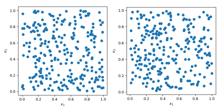
In both cases in the plot above, points are generated randomly without any knowledge about previously drawn points. It is clear that some regions of the space are left unexplored - which can cause problems in simulations as a particular set of points might trigger a totally different behavior.
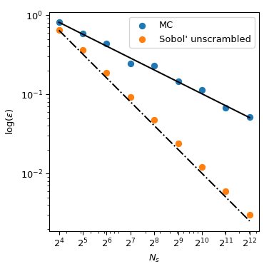
A great benefit of MC is that it has known convergence properties. Let’s look at the mean of the squared sum in 5 dimensions:
with \(x_j \sim \mathcal{U}(0,1)\). It has a known mean value, \(\mu = 5/3+5(5-1)/4\). Using MC sampling, we can compute that mean numerically, and the approximation error follows a theoretical rate of \(O(n^{-1/2})\).
Although the convergence is ensured, practitioners tend to want to have an exploration process that is more deterministic. With normal MC, a seed can be used to have a repeatable process. But fixing the seed would break the convergence property: a given seed could work for a given class of problem and break for another one.
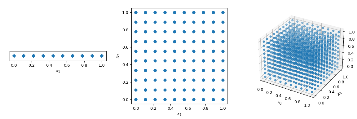
What is commonly done to walk through the space in a deterministic manner is to use a regular grid spanning all parameter dimensions, also called a saturated design. Let’s consider the unit-hypercube, with all bounds ranging from 0 to 1. Now, having a distance of 0.1 between points, the number of points required to fill the unit interval would be 10. In a 2-dimensional hypercube the same spacing would require 100, and in 3 dimensions 1,000 points. As the number of dimensions grows, the number of experiments required to fill the space rises exponentially as the dimensionality of the space increases. This exponential growth is called “the curse of dimensionality”.
>>> import numpy as np
>>> disc = 10
>>> x1 = np.linspace(0, 1, disc)
>>> x2 = np.linspace(0, 1, disc)
>>> x3 = np.linspace(0, 1, disc)
>>> x1, x2, x3 = np.meshgrid(x1, x2, x3)
To mitigate this issue, QMC methods have been designed. They are deterministic, have a good coverage of the space and some of them can be continued and retain good properties. The main difference with MC methods is that the points are not IID but they depend on previous points. Hence, some methods are also referred to as sequences.
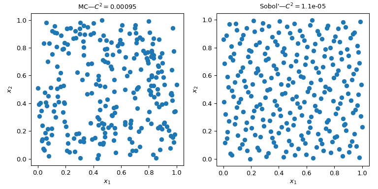
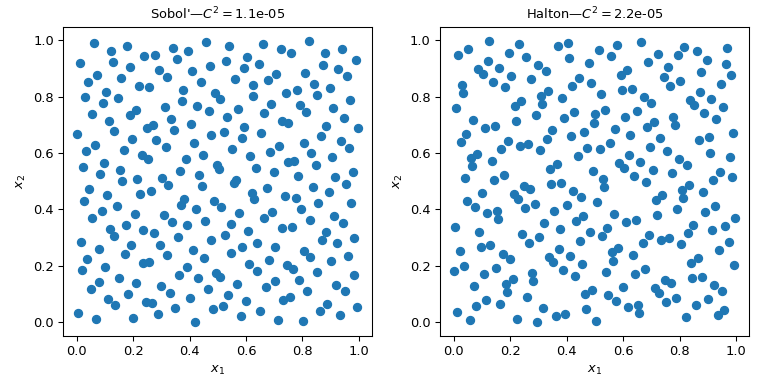
This figure presents 2 sets of 256 points. The design of the left is a plain MC whereas the design of the right is a QMC design using the Sobol’ method. We clearly see that the QMC version is more uniform. The points sample better near the boundaries and there are fewer clusters or gaps.
One way to assess the uniformity is to use a measure called discrepancy. Here the discrepancy of Sobol’ points is better than crude MC.
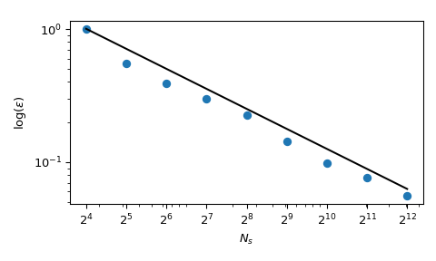
Coming back to the computation of the mean, QMC methods also have better rates of convergence for the error. They can achieve \(O(n^{-1})\) for this function, and even better rates on very smooth functions. This figure shows that the Sobol’ method has a rate of \(O(n^{-1})\):
We refer to the documentation of scipy.stats.qmc for
more mathematical details.
Calculate the discrepancy#
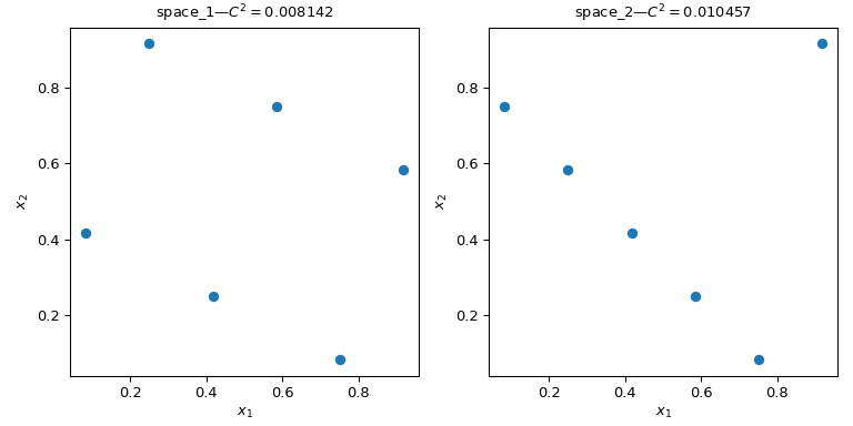
Let’s consider two sets of points. From the figure below, it is clear that
the design on the left covers more of the space than the design on the right.
This can be quantified using a scipy.stats.qmc.discrepancy measure.
The lower the discrepancy, the more uniform a sample is.
>>> import numpy as np
>>> from scipy.stats import qmc
>>> space_1 = np.array([[1, 3], [2, 6], [3, 2], [4, 5], [5, 1], [6, 4]])
>>> space_2 = np.array([[1, 5], [2, 4], [3, 3], [4, 2], [5, 1], [6, 6]])
>>> l_bounds = [0.5, 0.5]
>>> u_bounds = [6.5, 6.5]
>>> space_1 = qmc.scale(space_1, l_bounds, u_bounds, reverse=True)
>>> space_2 = qmc.scale(space_2, l_bounds, u_bounds, reverse=True)
>>> qmc.discrepancy(space_1)
0.008142039609053464
>>> qmc.discrepancy(space_2)
0.010456854423869011
Using a QMC engine#
Several QMC samplers/engines are implemented. Here we look at two of the most
used QMC methods: scipy.stats.qmc.Sobol and
scipy.stats.qmc.Halton sequences.
"""Sobol' and Halton sequences."""
from scipy.stats import qmc
import numpy as np

import matplotlib.pyplot as plt


rng = np.random.default_rng()

n_sample = 256
dim = 2

sample = {}

# Sobol'
engine = qmc.Sobol(d=dim, seed=rng)
sample["Sobol'"] = engine.random(n_sample)

# Halton
engine = qmc.Halton(d=dim, seed=rng)
sample["Halton"] = engine.random(n_sample)

fig, axs = plt.subplots(1, 2, figsize=(8, 4))

for i, kind in enumerate(sample):
    axs[i].scatter(sample[kind][:, 0], sample[kind][:, 1])

    axs[i].set_aspect('equal')
    axs[i].set_xlabel(r'$x_1$')
    axs[i].set_ylabel(r'$x_2$')
    axs[i].set_title(f'{kind}—$C^2 = ${qmc.discrepancy(sample[kind]):.2}')

plt.tight_layout()
plt.show()
Warning
QMC methods require particular care and the user must read the documentation to avoid common pitfalls. Sobol’ for instance requires a number of points following a power of 2. Also, thinning, burning or other point selection can break the properties of the sequence and result in a set of points which would not be better than MC.
QMC engines are state-aware. Meaning that you can continue the sequence,
skip some points, or reset it. Let’s take 5 points from
scipy.stats.qmc.Halton. And then ask for a second set of 5 points:
>>> from scipy.stats import qmc
>>> engine = qmc.Halton(d=2)
>>> engine.random(5)
array([[0.22166437, 0.07980522],  # random
       [0.72166437, 0.93165708],
       [0.47166437, 0.41313856],
       [0.97166437, 0.19091633],
       [0.01853937, 0.74647189]])
>>> engine.random(5)
array([[0.51853937, 0.52424967],  # random
       [0.26853937, 0.30202745],
       [0.76853937, 0.857583  ],
       [0.14353937, 0.63536078],
       [0.64353937, 0.01807683]])
Now we reset the sequence. Asking for 5 points leads to the same first 5 points:
>>> engine.reset()
>>> engine.random(5)
array([[0.22166437, 0.07980522],  # random
       [0.72166437, 0.93165708],
       [0.47166437, 0.41313856],
       [0.97166437, 0.19091633],
       [0.01853937, 0.74647189]])
And here we advance the sequence to get the same second set of 5 points:
>>> engine.reset()
>>> engine.fast_forward(5)
>>> engine.random(5)
array([[0.51853937, 0.52424967],  # random
       [0.26853937, 0.30202745],
       [0.76853937, 0.857583  ],
       [0.14353937, 0.63536078],
       [0.64353937, 0.01807683]])
Note
By default, both scipy.stats.qmc.Sobol and
scipy.stats.qmc.Halton are scrambled. The convergence properties are
better, and it prevents the appearance of fringes or noticeable patterns
of points in high dimensions. There should be no practical reason not to
use the scrambled version.
Making a QMC engine, i.e., subclassing QMCEngine#
To make your own scipy.stats.qmc.QMCEngine, a few methods have to be
defined. The following is an example wrapping numpy.random.Generator.
>>> import numpy as np
>>> from scipy.stats import qmc
>>> class RandomEngine(qmc.QMCEngine):
...     def __init__(self, d, seed=None):
...         super().__init__(d=d, seed=seed)
...         self.rng = np.random.default_rng(self.rng_seed)
...
...
...     def _random(self, n=1, *, workers=1):
...         return self.rng.random((n, self.d))
...
...
...     def reset(self):
...         self.rng = np.random.default_rng(self.rng_seed)
...         self.num_generated = 0
...         return self
...
...
...     def fast_forward(self, n):
...         self.random(n)
...         return self
Then we use it as any other QMC engine:
>>> engine = RandomEngine(2)
>>> engine.random(5)
array([[0.22733602, 0.31675834],  # random
       [0.79736546, 0.67625467],
       [0.39110955, 0.33281393],
       [0.59830875, 0.18673419],
       [0.67275604, 0.94180287]])
>>> engine.reset()
>>> engine.random(5)
array([[0.22733602, 0.31675834],  # random
       [0.79736546, 0.67625467],
       [0.39110955, 0.33281393],
       [0.59830875, 0.18673419],
       [0.67275604, 0.94180287]])
Guidelines on using QMC#
QMC has rules! Be sure to read the documentation or you might have no benefit over MC.
Use
scipy.stats.qmc.Sobolif you need exactly \(2^m\) points.scipy.stats.qmc.Haltonallows to sample, or skip, an arbitrary number of points. This is at the cost of a slower rate of convergence than Sobol’.Never remove the first points of the sequence. It will destroy the properties.
Scrambling is always better.
If you use LHS based methods, you cannot add points without losing the LHS properties. (There are some methods to do so, but this is not implemented.)