Kernel density estimation

A common task in statistics is to estimate the probability density function (PDF) of a random variable from a set of data samples. This task is called density estimation. The most well-known tool to do this is the histogram. A histogram is a useful tool for visualization (mainly because everyone understands it), but doesn’t use the available data very efficiently. Kernel density estimation (KDE) is a more efficient tool for the same task. The scipy.stats.gaussian_kde estimator can be used to estimate the PDF of univariate as well as multivariate data. It works best if the data is unimodal.

Univariate estimation

We start with a minimal amount of data in order to see how scipy.stats.gaussian_kde works and what the different options for bandwidth selection do. The data sampled from the PDF are shown as blue dashes at the bottom of the figure (this is called a rug plot):

>>> from scipy import stats
>>> import matplotlib.pyplot as plt

>>> x1 = np.array([-7, -5, 1, 4, 5], dtype=np.float64)
>>> kde1 = stats.gaussian_kde(x1)
>>> kde2 = stats.gaussian_kde(x1, bw_method='silverman')

>>> fig = plt.figure()
>>> ax = fig.add_subplot(111)

>>> ax.plot(x1, np.zeros(x1.shape), 'b+', ms=20)  # rug plot
>>> x_eval = np.linspace(-10, 10, num=200)
>>> ax.plot(x_eval, kde1(x_eval), 'k-', label="Scott's Rule")
>>> ax.plot(x_eval, kde2(x_eval), 'r-', label="Silverman's Rule")

>>> plt.show()

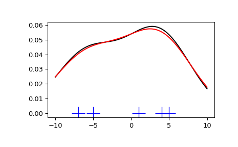
We see that there is very little difference between Scott’s Rule and Silverman’s Rule, and that the bandwidth selection with a limited amount of data is probably a bit too wide. We can define our own bandwidth function to get a less smoothed-out result.

>>> def my_kde_bandwidth(obj, fac=1./5):
...     """We use Scott's Rule, multiplied by a constant factor."""
...     return np.power(obj.n, -1./(obj.d+4)) * fac

>>> fig = plt.figure()
>>> ax = fig.add_subplot(111)

>>> ax.plot(x1, np.zeros(x1.shape), 'b+', ms=20)  # rug plot
>>> kde3 = stats.gaussian_kde(x1, bw_method=my_kde_bandwidth)
>>> ax.plot(x_eval, kde3(x_eval), 'g-', label="With smaller BW")

>>> plt.show()

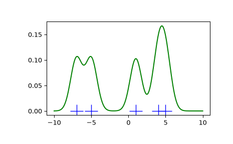
We see that if we set bandwidth to be very narrow, the obtained estimate for the probability density function (PDF) is simply the sum of Gaussians around each data point.

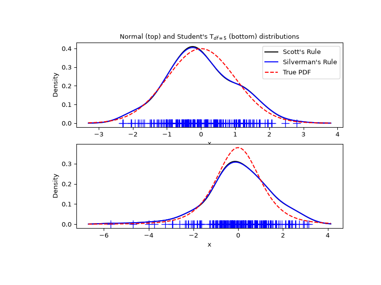
We now take a more realistic example and look at the difference between the two available bandwidth selection rules. Those rules are known to work well for (close to) normal distributions, but even for unimodal distributions that are quite strongly non-normal they work reasonably well. As a non-normal distribution we take a Student’s T distribution with 5 degrees of freedom.

import numpy as np
import matplotlib.pyplot as plt
from scipy import stats


rng = np.random.default_rng()
x1 = rng.normal(size=200)  # random data, normal distribution
xs = np.linspace(x1.min()-1, x1.max()+1, 200)

kde1 = stats.gaussian_kde(x1)
kde2 = stats.gaussian_kde(x1, bw_method='silverman')

fig = plt.figure(figsize=(8, 6))

ax1 = fig.add_subplot(211)
ax1.plot(x1, np.zeros(x1.shape), 'b+', ms=12)  # rug plot
ax1.plot(xs, kde1(xs), 'k-', label="Scott's Rule")
ax1.plot(xs, kde2(xs), 'b-', label="Silverman's Rule")
ax1.plot(xs, stats.norm.pdf(xs), 'r--', label="True PDF")

ax1.set_xlabel('x')
ax1.set_ylabel('Density')
ax1.set_title("Normal (top) and Student's T$_{df=5}$ (bottom) distributions")
ax1.legend(loc=1)

x2 = stats.t.rvs(5, size=200, random_state=rng)  # random data, T distribution
xs = np.linspace(x2.min() - 1, x2.max() + 1, 200)

kde3 = stats.gaussian_kde(x2)
kde4 = stats.gaussian_kde(x2, bw_method='silverman')

ax2 = fig.add_subplot(212)
ax2.plot(x2, np.zeros(x2.shape), 'b+', ms=12)  # rug plot
ax2.plot(xs, kde3(xs), 'k-', label="Scott's Rule")
ax2.plot(xs, kde4(xs), 'b-', label="Silverman's Rule")
ax2.plot(xs, stats.t.pdf(xs, 5), 'r--', label="True PDF")

ax2.set_xlabel('x')
ax2.set_ylabel('Density')

plt.show()

We now take a look at a bimodal distribution with one wider and one narrower Gaussian feature. We expect that this will be a more difficult density to approximate, due to the different bandwidths required to accurately resolve each feature.

>>> from functools import partial

>>> loc1, scale1, size1 = (-2, 1, 175)
>>> loc2, scale2, size2 = (2, 0.2, 50)
>>> x2 = np.concatenate([np.random.normal(loc=loc1, scale=scale1, size=size1),
...                      np.random.normal(loc=loc2, scale=scale2, size=size2)])

>>> x_eval = np.linspace(x2.min() - 1, x2.max() + 1, 500)

>>> kde = stats.gaussian_kde(x2)
>>> kde2 = stats.gaussian_kde(x2, bw_method='silverman')
>>> kde3 = stats.gaussian_kde(x2, bw_method=partial(my_kde_bandwidth, fac=0.2))
>>> kde4 = stats.gaussian_kde(x2, bw_method=partial(my_kde_bandwidth, fac=0.5))

>>> pdf = stats.norm.pdf
>>> bimodal_pdf = pdf(x_eval, loc=loc1, scale=scale1) * float(size1) / x2.size + \
...               pdf(x_eval, loc=loc2, scale=scale2) * float(size2) / x2.size

>>> fig = plt.figure(figsize=(8, 6))
>>> ax = fig.add_subplot(111)

>>> ax.plot(x2, np.zeros(x2.shape), 'b+', ms=12)
>>> ax.plot(x_eval, kde(x_eval), 'k-', label="Scott's Rule")
>>> ax.plot(x_eval, kde2(x_eval), 'b-', label="Silverman's Rule")
>>> ax.plot(x_eval, kde3(x_eval), 'g-', label="Scott * 0.2")
>>> ax.plot(x_eval, kde4(x_eval), 'c-', label="Scott * 0.5")
>>> ax.plot(x_eval, bimodal_pdf, 'r--', label="Actual PDF")

>>> ax.set_xlim([x_eval.min(), x_eval.max()])
>>> ax.legend(loc=2)
>>> ax.set_xlabel('x')
>>> ax.set_ylabel('Density')
>>> plt.show()

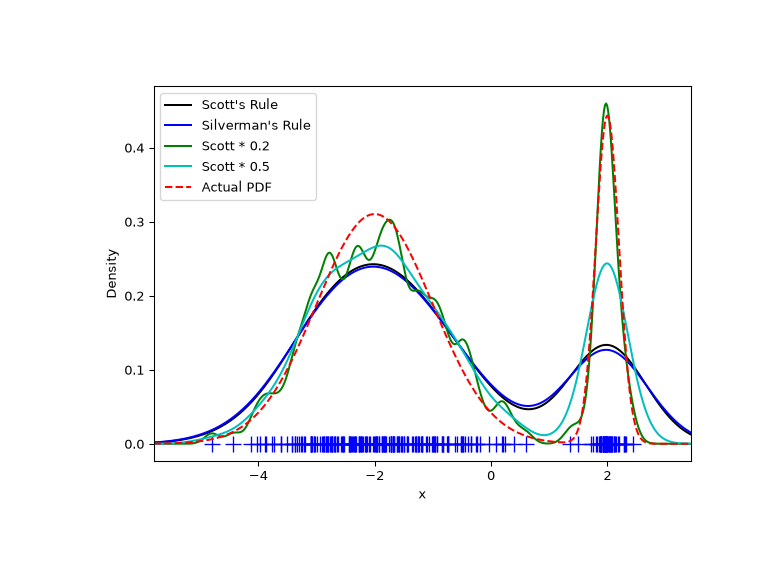
As expected, the KDE is not as close to the true PDF as we would like due to the different characteristic size of the two features of the bimodal distribution. By halving the default bandwidth (Scott * 0.5), we can do somewhat better, while using a factor 5 smaller bandwidth than the default doesn’t smooth enough. What we really need, though, in this case, is a non-uniform (adaptive) bandwidth.

Multivariate estimation

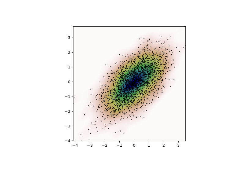
With scipy.stats.gaussian_kde we can perform multivariate, as well as univariate estimation. We demonstrate the bivariate case. First, we generate some random data with a model in which the two variates are correlated.

>>> def measure(n):
...     """Measurement model, return two coupled measurements."""
...     m1 = np.random.normal(size=n)
...     m2 = np.random.normal(scale=0.5, size=n)
...     return m1+m2, m1-m2

>>> m1, m2 = measure(2000)
>>> xmin = m1.min()
>>> xmax = m1.max()
>>> ymin = m2.min()
>>> ymax = m2.max()

Then we apply the KDE to the data:

>>> X, Y = np.mgrid[xmin:xmax:100j, ymin:ymax:100j]
>>> positions = np.vstack([X.ravel(), Y.ravel()])
>>> values = np.vstack([m1, m2])
>>> kernel = stats.gaussian_kde(values)
>>> Z = np.reshape(kernel.evaluate(positions).T, X.shape)

Finally, we plot the estimated bivariate distribution as a colormap and plot the individual data points on top.

>>> fig = plt.figure(figsize=(8, 6))
>>> ax = fig.add_subplot(111)

>>> ax.imshow(np.rot90(Z), cmap=plt.cm.gist_earth_r,
...           extent=[xmin, xmax, ymin, ymax])
>>> ax.plot(m1, m2, 'k.', markersize=2)

>>> ax.set_xlim([xmin, xmax])
>>> ax.set_ylim([ymin, ymax])

>>> plt.show()