Levene test for equal variances#
The Levene test scipy.stats.levene tests the null hypothesis that all
input samples are from populations with equal variances. Levene’s test is an
alternative to Bartlett’s test scipy.stats.bartlett in the case where
there are significant deviations from normality.
In [1], the influence of vitamin C on the tooth growth of guinea pigs was investigated. In a control study, 60 subjects were divided into small dose, medium dose, and large dose groups that received daily doses of 0.5, 1.0 and 2.0 mg of vitamin C, respectively. After 42 days, the tooth growth was measured.
The small_dose, medium_dose, and large_dose arrays below record
tooth growth measurements of the three groups in microns.
import numpy as np
small_dose = np.array([
    4.2, 11.5, 7.3, 5.8, 6.4, 10, 11.2, 11.2, 5.2, 7,
    15.2, 21.5, 17.6, 9.7, 14.5, 10, 8.2, 9.4, 16.5, 9.7
])
medium_dose = np.array([
    16.5, 16.5, 15.2, 17.3, 22.5, 17.3, 13.6, 14.5, 18.8, 15.5,
    19.7, 23.3, 23.6, 26.4, 20, 25.2, 25.8, 21.2, 14.5, 27.3
])
large_dose = np.array([
    23.6, 18.5, 33.9, 25.5, 26.4, 32.5, 26.7, 21.5, 23.3, 29.5,
    25.5, 26.4, 22.4, 24.5, 24.8, 30.9, 26.4, 27.3, 29.4, 23
])
The scipy.stats.levene statistic is sensitive to differences in
variances between the samples.
from scipy import stats
res = stats.levene(small_dose, medium_dose, large_dose)
res.statistic
np.float64(0.6457341109631506)
The value of the statistic tends to be high when there is a large difference in variances.
We can test for inequality of variance among the groups by comparing the observed value of the statistic against the null distribution: the distribution of statistic values derived under the null hypothesis that the population variances of the three groups are equal.
For this test, the null distribution follows the F distribution as shown below.
import matplotlib.pyplot as plt
k, n = 3, 60   # number of samples, total number of observations
dist = stats.f(dfn=k-1, dfd=n-k)
val = np.linspace(0, 5, 100)
pdf = dist.pdf(val)
fig, ax = plt.subplots(figsize=(8, 5))

def plot(ax):  # we'll reuse this
    ax.plot(val, pdf, color='C0')
    ax.set_title("Levene Test Null Distribution")
    ax.set_xlabel("statistic")
    ax.set_ylabel("probability density")
    ax.set_xlim(0, 5)
    ax.set_ylim(0, 1)

plot(ax)
plt.show()

The comparison is quantified by the p-value: the proportion of values in the null distribution greater than or equal to the observed value of the statistic.
fig, ax = plt.subplots(figsize=(8, 5))
plot(ax)
pvalue = dist.sf(res.statistic)
annotation = (f'p-value={pvalue:.3f}\n(shaded area)')
props = dict(facecolor='black', width=1, headwidth=5, headlength=8)
_ = ax.annotate(annotation, (1.5, 0.22), (2.25, 0.3), arrowprops=props)
i = val >= res.statistic
ax.fill_between(val[i], y1=0, y2=pdf[i], color='C0')
plt.show()

res.pvalue
np.float64(0.5280694573759913)
If the p-value is “small” - that is, if there is a low probability of sampling data from distributions with identical variances that produces such an extreme value of the statistic - this may be taken as evidence against the null hypothesis in favor of the alternative: the variances of the groups are not equal. Note that:
The inverse is not true; that is, the test is not used to provide evidence for the null hypothesis.
The threshold for values that will be considered “small” is a choice that should be made before the data is analyzed [2] with consideration of the risks of both false positives (incorrectly rejecting the null hypothesis) and false negatives (failure to reject a false null hypothesis).
Small p-values are not evidence for a large effect; rather, they can only provide evidence for a “significant” effect, meaning that they are unlikely to have occurred under the null hypothesis.
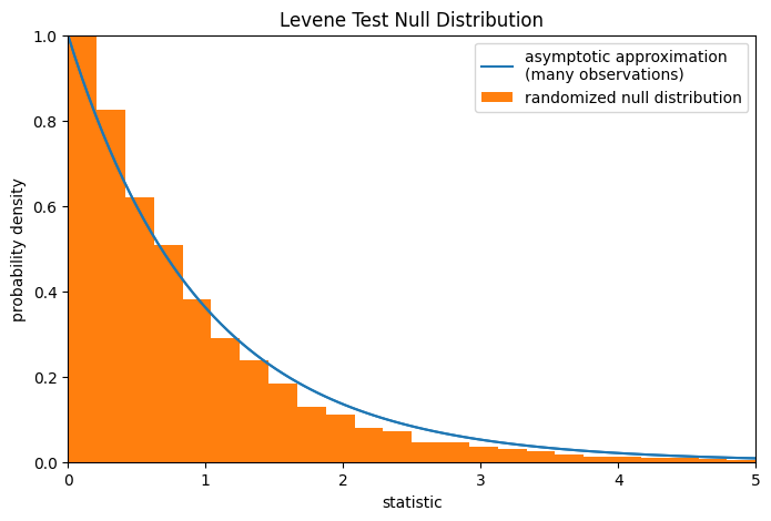
Note that the F distribution provides an asymptotic approximation of the null distribution. For small samples, it may be more appropriate to perform a permutation test: Under the null hypothesis that all three samples were drawn from the same population, each of the measurements is equally likely to have been observed in any of the three samples. Therefore, we can form a randomized null distribution by calculating the statistic under many randomly-generated partitionings of the observations into the three samples.
def statistic(*samples):
    return stats.levene(*samples).statistic
ref = stats.permutation_test(
    (small_dose, medium_dose, large_dose), statistic,
    permutation_type='independent', alternative='greater'
)
fig, ax = plt.subplots(figsize=(8, 5))
plot(ax)
bins = np.linspace(0, 5, 25)
ax.hist(
    ref.null_distribution, bins=bins, density=True, facecolor="C1"
)
ax.legend(['asymptotic approximation\n(many observations)',
           'randomized null distribution'])
plot(ax)
plt.show()
ref.pvalue # randomized test p-value
np.float64(0.4584)
Note that there is significant disagreement between the p-value calculated here
and the asymptotic approximation returned by scipy.stats.levene above.
The statistical inferences that can be drawn rigorously from a permutation test
are limited; nonetheless, they may be the preferred approach in many
circumstances [3].