scipy.stats.zipfian#

scipy.stats.zipfian = <scipy.stats._discrete_distns.zipfian_gen object>[source]#

A Zipfian discrete random variable.

As an instance of the rv_discrete class, zipfian object inherits from it a collection of generic methods (see below for the full list), and completes them with details specific for this particular distribution.

Methods

rvs(a, n, loc=0, size=1, random_state=None)	Random variates.
pmf(k, a, n, loc=0)	Probability mass function.
logpmf(k, a, n, loc=0)	Log of the probability mass function.
cdf(k, a, n, loc=0)	Cumulative distribution function.
logcdf(k, a, n, loc=0)	Log of the cumulative distribution function.
sf(k, a, n, loc=0)	Survival function (also defined as `1 - cdf`, but sf is sometimes more accurate).
logsf(k, a, n, loc=0)	Log of the survival function.
ppf(q, a, n, loc=0)	Percent point function (inverse of `cdf` — percentiles).
isf(q, a, n, loc=0)	Inverse survival function (inverse of `sf`).
stats(a, n, loc=0, moments=’mv’)	Mean(‘m’), variance(‘v’), skew(‘s’), and/or kurtosis(‘k’).
entropy(a, n, loc=0)	(Differential) entropy of the RV.
expect(func, args=(a, n), loc=0, lb=None, ub=None, conditional=False)	Expected value of a function (of one argument) with respect to the distribution.
median(a, n, loc=0)	Median of the distribution.
mean(a, n, loc=0)	Mean of the distribution.
var(a, n, loc=0)	Variance of the distribution.
std(a, n, loc=0)	Standard deviation of the distribution.
interval(confidence, a, n, loc=0)	Confidence interval with equal areas around the median.

See also

zipf

Notes

The probability mass function for zipfian is:

\[f(k, a, n) = \frac{1}{H_{n,a} k^a}\]

for \(k \in \{1, 2, \dots, n-1, n\}\), \(a \ge 0\), \(n \in \{1, 2, 3, \dots\}\).

zipfian takes \(a\) and \(n\) as shape parameters. \(H_{n,a}\) is the \(n\)^th generalized harmonic number of order \(a\).

The Zipfian distribution reduces to the Zipf (zeta) distribution as \(n \rightarrow \infty\).

The probability mass function above is defined in the “standardized” form. To shift distribution use the loc parameter. Specifically, zipfian.pmf(k, a, n, loc) is identically equivalent to zipfian.pmf(k - loc, a, n).

References

[1]

“Zipf’s Law”, Wikipedia, https://en.wikipedia.org/wiki/Zipf’s_law

[2]

Larry Leemis, “Zipf Distribution”, Univariate Distribution Relationships. http://www.math.wm.edu/~leemis/chart/UDR/PDFs/Zipf.pdf

Examples

>>> import numpy as np
>>> from scipy.stats import zipfian
>>> import matplotlib.pyplot as plt
>>> fig, ax = plt.subplots(1, 1)

Calculate the first four moments:

>>> a, n = 1.25, 10
>>> mean, var, skew, kurt = zipfian.stats(a, n, moments='mvsk')

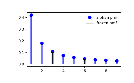
Display the probability mass function (pmf):

>>> x = np.arange(zipfian.ppf(0.01, a, n),
...               zipfian.ppf(0.99, a, n))
>>> ax.plot(x, zipfian.pmf(x, a, n), 'bo', ms=8, label='zipfian pmf')
>>> ax.vlines(x, 0, zipfian.pmf(x, a, n), colors='b', lw=5, alpha=0.5)

Alternatively, the distribution object can be called (as a function) to fix the shape and location. This returns a “frozen” RV object holding the given parameters fixed.

Freeze the distribution and display the frozen pmf:

>>> rv = zipfian(a, n)
>>> ax.vlines(x, 0, rv.pmf(x), colors='k', linestyles='-', lw=1,
...         label='frozen pmf')
>>> ax.legend(loc='best', frameon=False)
>>> plt.show()

../../_images/scipy-stats-zipfian-1_00_00.png

Check accuracy of cdf and ppf:

>>> prob = zipfian.cdf(x, a, n)
>>> np.allclose(x, zipfian.ppf(prob, a, n))
True

Generate random numbers:

>>> r = zipfian.rvs(a, n, size=1000)

Confirm that zipfian reduces to zipf for large n, a > 1.

>>> import numpy as np
>>> from scipy.stats import zipf, zipfian
>>> k = np.arange(11)
>>> np.allclose(zipfian.pmf(k, a=3.5, n=10000000), zipf.pmf(k, a=3.5))
True