scipy.stats.

yeojohnson#

scipy.stats.yeojohnson(x, lmbda=None)[source]#

Return a dataset transformed by a Yeo-Johnson power transformation.

Parameters:

xndarray: Input array. Should be 1-dimensional.
lmbdafloat, optional: If lmbda is None, find the lambda that maximizes the log-likelihood function and return it as the second output argument. Otherwise the transformation is done for the given value.

Returns:

yeojohnson: ndarray: Yeo-Johnson power transformed array.
maxlogfloat, optional: If the lmbda parameter is None, the second returned argument is the lambda that maximizes the log-likelihood function.

See also

probplot, yeojohnson_normplot, yeojohnson_normmax, yeojohnson_llf, boxcox

Notes

The Yeo-Johnson transform is given by:

y = ((x + 1)**lmbda - 1) / lmbda,                for x >= 0, lmbda != 0
    log(x + 1),                                  for x >= 0, lmbda = 0
    -((-x + 1)**(2 - lmbda) - 1) / (2 - lmbda),  for x < 0, lmbda != 2
    -log(-x + 1),                                for x < 0, lmbda = 2

Unlike boxcox, yeojohnson does not require the input data to be positive.

Added in version 1.2.0.

References

I. Yeo and R.A. Johnson, “A New Family of Power Transformations to Improve Normality or Symmetry”, Biometrika 87.4 (2000):

Examples

>>> from scipy import stats
>>> import matplotlib.pyplot as plt

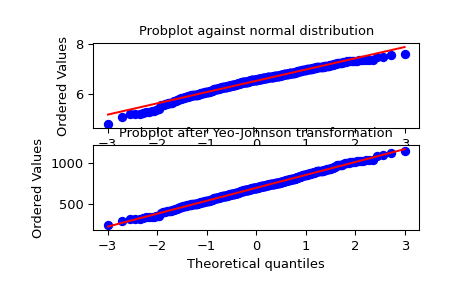
We generate some random variates from a non-normal distribution and make a probability plot for it, to show it is non-normal in the tails:

>>> fig = plt.figure()
>>> ax1 = fig.add_subplot(211)
>>> x = stats.loggamma.rvs(5, size=500) + 5
>>> prob = stats.probplot(x, dist=stats.norm, plot=ax1)
>>> ax1.set_xlabel('')
>>> ax1.set_title('Probplot against normal distribution')

We now use yeojohnson to transform the data so it’s closest to normal:

>>> ax2 = fig.add_subplot(212)
>>> xt, lmbda = stats.yeojohnson(x)
>>> prob = stats.probplot(xt, dist=stats.norm, plot=ax2)
>>> ax2.set_title('Probplot after Yeo-Johnson transformation')

>>> plt.show()

../../_images/scipy-stats-yeojohnson-1.png