scipy.stats.vonmises_fisher#
- scipy.stats.vonmises_fisher = <scipy.stats._multivariate.vonmises_fisher_gen object>[source]#
A von Mises-Fisher variable.
The mu keyword specifies the mean direction vector. The kappa keyword specifies the concentration parameter.
- Parameters:
- muarray_like
Mean direction of the distribution. Must be a one-dimensional unit vector of norm 1.
- kappafloat
Concentration parameter. Must be positive.
- seed{None, int, np.random.RandomState, np.random.Generator}, optional
Used for drawing random variates. If seed is None, the RandomState singleton is used. If seed is an int, a new
RandomStateinstance is used, seeded with seed. If seed is already aRandomStateorGeneratorinstance, then that object is used. Default is None.
Methods
pdf(x, mu=None, kappa=1)
Probability density function.
logpdf(x, mu=None, kappa=1)
Log of the probability density function.
rvs(mu=None, kappa=1, size=1, random_state=None)
Draw random samples from a von Mises-Fisher distribution.
entropy(mu=None, kappa=1)
Compute the differential entropy of the von Mises-Fisher distribution.
fit(data)
Fit a von Mises-Fisher distribution to data.
See also
scipy.stats.vonmisesVon-Mises Fisher distribution in 2D on a circle
uniform_directionuniform distribution on the surface of a hypersphere
Notes
The von Mises-Fisher distribution is a directional distribution on the surface of the unit hypersphere. The probability density function of a unit vector \(\mathbf{x}\) is
\[f(\mathbf{x}) = \frac{\kappa^{d/2-1}}{(2\pi)^{d/2}I_{d/2-1}(\kappa)} \exp\left(\kappa \mathbf{\mu}^T\mathbf{x}\right),\]where \(\mathbf{\mu}\) is the mean direction, \(\kappa\) the concentration parameter, \(d\) the dimension and \(I\) the modified Bessel function of the first kind. As \(\mu\) represents a direction, it must be a unit vector or in other words, a point on the hypersphere: \(\mathbf{\mu}\in S^{d-1}\). \(\kappa\) is a concentration parameter, which means that it must be positive (\(\kappa>0\)) and that the distribution becomes more narrow with increasing \(\kappa\). In that sense, the reciprocal value \(1/\kappa\) resembles the variance parameter of the normal distribution.
The von Mises-Fisher distribution often serves as an analogue of the normal distribution on the sphere. Intuitively, for unit vectors, a useful distance measure is given by the angle \(\alpha\) between them. This is exactly what the scalar product \(\mathbf{\mu}^T\mathbf{x}=\cos(\alpha)\) in the von Mises-Fisher probability density function describes: the angle between the mean direction \(\mathbf{\mu}\) and the vector \(\mathbf{x}\). The larger the angle between them, the smaller the probability to observe \(\mathbf{x}\) for this particular mean direction \(\mathbf{\mu}\).
In dimensions 2 and 3, specialized algorithms are used for fast sampling [2], [3]. For dimensions of 4 or higher the rejection sampling algorithm described in [4] is utilized. This implementation is partially based on the geomstats package [5], [6].
Added in version 1.11.
References
[1]Von Mises-Fisher distribution, Wikipedia, https://en.wikipedia.org/wiki/Von_Mises%E2%80%93Fisher_distribution
[2]Mardia, K., and Jupp, P. Directional statistics. Wiley, 2000.
[3]J. Wenzel. Numerically stable sampling of the von Mises Fisher distribution on S2. https://www.mitsuba-renderer.org/~wenzel/files/vmf.pdf
[4]Wood, A. Simulation of the von mises fisher distribution. Communications in statistics-simulation and computation 23, 1 (1994), 157-164. DOI:10.1080/03610919408813161.
[5]geomstats, Github. MIT License. Accessed: 06.01.2023. geomstats/geomstats
[6]Miolane, N. et al. Geomstats: A Python Package for Riemannian Geometry in Machine Learning. Journal of Machine Learning Research 21 (2020). http://jmlr.org/papers/v21/19-027.html
Examples
Visualization of the probability density
Plot the probability density in three dimensions for increasing concentration parameter. The density is calculated by the
pdfmethod.>>> import numpy as np >>> import matplotlib.pyplot as plt >>> from scipy.stats import vonmises_fisher >>> from matplotlib.colors import Normalize >>> n_grid = 100 >>> u = np.linspace(0, np.pi, n_grid) >>> v = np.linspace(0, 2 * np.pi, n_grid) >>> u_grid, v_grid = np.meshgrid(u, v) >>> vertices = np.stack([np.cos(v_grid) * np.sin(u_grid), ... np.sin(v_grid) * np.sin(u_grid), ... np.cos(u_grid)], ... axis=2) >>> x = np.outer(np.cos(v), np.sin(u)) >>> y = np.outer(np.sin(v), np.sin(u)) >>> z = np.outer(np.ones_like(u), np.cos(u)) >>> def plot_vmf_density(ax, x, y, z, vertices, mu, kappa): ... vmf = vonmises_fisher(mu, kappa) ... pdf_values = vmf.pdf(vertices) ... pdfnorm = Normalize(vmin=pdf_values.min(), vmax=pdf_values.max()) ... ax.plot_surface(x, y, z, rstride=1, cstride=1, ... facecolors=plt.cm.viridis(pdfnorm(pdf_values)), ... linewidth=0) ... ax.set_aspect('equal') ... ax.view_init(azim=-130, elev=0) ... ax.axis('off') ... ax.set_title(rf"$\kappa={kappa}$") >>> fig, axes = plt.subplots(nrows=1, ncols=3, figsize=(9, 4), ... subplot_kw={"projection": "3d"}) >>> left, middle, right = axes >>> mu = np.array([-np.sqrt(0.5), -np.sqrt(0.5), 0]) >>> plot_vmf_density(left, x, y, z, vertices, mu, 5) >>> plot_vmf_density(middle, x, y, z, vertices, mu, 20) >>> plot_vmf_density(right, x, y, z, vertices, mu, 100) >>> plt.subplots_adjust(top=1, bottom=0.0, left=0.0, right=1.0, wspace=0.) >>> plt.show()
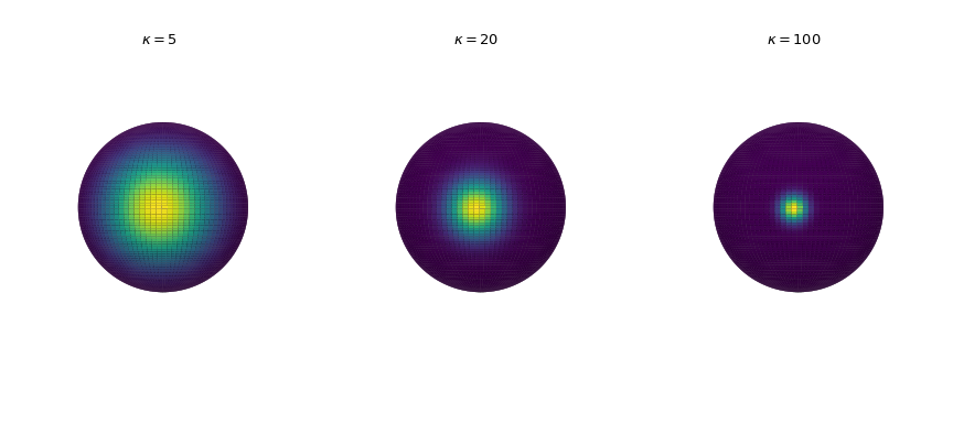
As we increase the concentration parameter, the points are getting more clustered together around the mean direction.
Sampling
Draw 5 samples from the distribution using the
rvsmethod resulting in a 5x3 array.>>> rng = np.random.default_rng() >>> mu = np.array([0, 0, 1]) >>> samples = vonmises_fisher(mu, 20).rvs(5, random_state=rng) >>> samples array([[ 0.3884594 , -0.32482588, 0.86231516], [ 0.00611366, -0.09878289, 0.99509023], [-0.04154772, -0.01637135, 0.99900239], [-0.14613735, 0.12553507, 0.98126695], [-0.04429884, -0.23474054, 0.97104814]])
These samples are unit vectors on the sphere \(S^2\). To verify, let us calculate their euclidean norms:
>>> np.linalg.norm(samples, axis=1)
array([1., 1., 1., 1., 1.])
Plot 20 observations drawn from the von Mises-Fisher distribution for increasing concentration parameter \(\kappa\). The red dot highlights the mean direction \(\mu\).
>>> def plot_vmf_samples(ax, x, y, z, mu, kappa):
...     vmf = vonmises_fisher(mu, kappa)
...     samples = vmf.rvs(20)
...     ax.plot_surface(x, y, z, rstride=1, cstride=1, linewidth=0,
...                     alpha=0.2)
...     ax.scatter(samples[:, 0], samples[:, 1], samples[:, 2], c='k', s=5)
...     ax.scatter(mu[0], mu[1], mu[2], c='r', s=30)
...     ax.set_aspect('equal')
...     ax.view_init(azim=-130, elev=0)
...     ax.axis('off')
...     ax.set_title(rf"$\kappa={kappa}$")
>>> mu = np.array([-np.sqrt(0.5), -np.sqrt(0.5), 0])
>>> fig, axes = plt.subplots(nrows=1, ncols=3,
...                          subplot_kw={"projection": "3d"},
...                          figsize=(9, 4))
>>> left, middle, right = axes
>>> plot_vmf_samples(left, x, y, z, mu, 5)
>>> plot_vmf_samples(middle, x, y, z, mu, 20)
>>> plot_vmf_samples(right, x, y, z, mu, 100)
>>> plt.subplots_adjust(top=1, bottom=0.0, left=0.0,
...                     right=1.0, wspace=0.)
>>> plt.show()
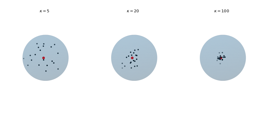
The plots show that with increasing concentration \(\kappa\) the resulting samples are centered more closely around the mean direction.
Fitting the distribution parameters
The distribution can be fitted to data using the
fitmethod returning the estimated parameters. As a toy example let’s fit the distribution to samples drawn from a known von Mises-Fisher distribution.>>> mu, kappa = np.array([0, 0, 1]), 20 >>> samples = vonmises_fisher(mu, kappa).rvs(1000, random_state=rng) >>> mu_fit, kappa_fit = vonmises_fisher.fit(samples) >>> mu_fit, kappa_fit (array([0.01126519, 0.01044501, 0.99988199]), 19.306398751730995)
We see that the estimated parameters mu_fit and kappa_fit are very close to the ground truth parameters.