scipy.stats.truncpareto

scipy.stats.truncpareto = <scipy.stats._continuous_distns.truncpareto_gen object>

An upper truncated Pareto continuous random variable.

As an instance of the rv_continuous class, truncpareto object inherits from it a collection of generic methods (see below for the full list), and completes them with details specific for this particular distribution.

Methods

rvs(b, c, loc=0, scale=1, size=1, random_state=None)	Random variates.
pdf(x, b, c, loc=0, scale=1)	Probability density function.
logpdf(x, b, c, loc=0, scale=1)	Log of the probability density function.
cdf(x, b, c, loc=0, scale=1)	Cumulative distribution function.
logcdf(x, b, c, loc=0, scale=1)	Log of the cumulative distribution function.
sf(x, b, c, loc=0, scale=1)	Survival function (also defined as 1 - cdf, but sf is sometimes more accurate).
logsf(x, b, c, loc=0, scale=1)	Log of the survival function.
ppf(q, b, c, loc=0, scale=1)	Percent point function (inverse of cdf — percentiles).
isf(q, b, c, loc=0, scale=1)	Inverse survival function (inverse of sf).
moment(order, b, c, loc=0, scale=1)	Non-central moment of the specified order.
stats(b, c, loc=0, scale=1, moments=’mv’)	Mean(‘m’), variance(‘v’), skew(‘s’), and/or kurtosis(‘k’).
entropy(b, c, loc=0, scale=1)	(Differential) entropy of the RV.
fit(data)	Parameter estimates for generic data. See scipy.stats.rv_continuous.fit for detailed documentation of the keyword arguments.
expect(func, args=(b, c), loc=0, scale=1, lb=None, ub=None, conditional=False, **kwds)	Expected value of a function (of one argument) with respect to the distribution.
median(b, c, loc=0, scale=1)	Median of the distribution.
mean(b, c, loc=0, scale=1)	Mean of the distribution.
var(b, c, loc=0, scale=1)	Variance of the distribution.
std(b, c, loc=0, scale=1)	Standard deviation of the distribution.
interval(confidence, b, c, loc=0, scale=1)	Confidence interval with equal areas around the median.

See also

pareto

Pareto distribution

Notes

The probability density function for truncpareto is:

\[f(x, b, c) = \frac{b}{1 - c^{-b}} \frac{1}{x^{b+1}}\]

for \(b > 0\), \(c > 1\) and \(1 \le x \le c\).

truncpareto takes b and c as shape parameters for \(b\) and \(c\).

Notice that the upper truncation value \(c\) is defined in standardized form so that random values of an unscaled, unshifted variable are within the range [1, c]. If u_r is the upper bound to a scaled and/or shifted variable, then c = (u_r - loc) / scale. In other words, the support of the distribution becomes (scale + loc) <= x <= (c*scale + loc) when scale and/or loc are provided.

The probability density above is defined in the “standardized” form. To shift and/or scale the distribution use the loc and scale parameters. Specifically, truncpareto.pdf(x, b, c, loc, scale) is identically equivalent to truncpareto.pdf(y, b, c) / scale with y = (x - loc) / scale. Note that shifting the location of a distribution does not make it a “noncentral” distribution; noncentral generalizations of some distributions are available in separate classes.

References

[1]

Burroughs, S. M., and Tebbens S. F. “Upper-truncated power laws in natural systems.” Pure and Applied Geophysics 158.4 (2001): 741-757.

Examples

Try it in your browser!

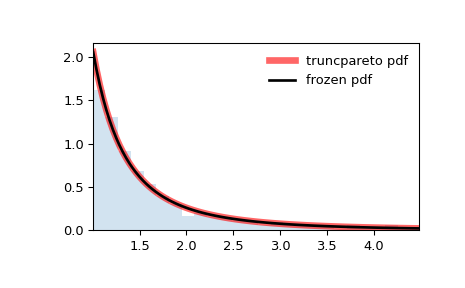
>>> import numpy as np
>>> from scipy.stats import truncpareto
>>> import matplotlib.pyplot as plt
>>> fig, ax = plt.subplots(1, 1)

Get the support:

>>> b, c = 2, 5
>>> lb, ub = truncpareto.support(b, c)

Calculate the first four moments:

>>> mean, var, skew, kurt = truncpareto.stats(b, c, moments='mvsk')

Display the probability density function (pdf):

>>> x = np.linspace(truncpareto.ppf(0.01, b, c),
...                 truncpareto.ppf(0.99, b, c), 100)
>>> ax.plot(x, truncpareto.pdf(x, b, c),
...        'r-', lw=5, alpha=0.6, label='truncpareto pdf')

Alternatively, the distribution object can be called (as a function) to fix the shape, location and scale parameters. This returns a “frozen” RV object holding the given parameters fixed.

Freeze the distribution and display the frozen pdf:

>>> rv = truncpareto(b, c)
>>> ax.plot(x, rv.pdf(x), 'k-', lw=2, label='frozen pdf')

Check accuracy of cdf and ppf:

>>> vals = truncpareto.ppf([0.001, 0.5, 0.999], b, c)
>>> np.allclose([0.001, 0.5, 0.999], truncpareto.cdf(vals, b, c))
True

Generate random numbers:

>>> r = truncpareto.rvs(b, c, size=1000)

And compare the histogram:

>>> ax.hist(r, density=True, bins='auto', histtype='stepfilled', alpha=0.2)
>>> ax.set_xlim([x[0], x[-1]])
>>> ax.legend(loc='best', frameon=False)
>>> plt.show()

Go BackOpen In Tab