scipy.stats.ksone#
- scipy.stats.ksone = <scipy.stats._continuous_distns.ksone_gen object>[source]#
Kolmogorov-Smirnov one-sided test statistic distribution.
This is the distribution of the one-sided Kolmogorov-Smirnov (KS) statistics \(D_n^+\) and \(D_n^-\) for a finite sample size
n >= 1(the shape parameter).As an instance of the
rv_continuousclass,ksoneobject inherits from it a collection of generic methods (see below for the full list), and completes them with details specific for this particular distribution.Methods
rvs(n, loc=0, scale=1, size=1, random_state=None)
Random variates.
pdf(x, n, loc=0, scale=1)
Probability density function.
logpdf(x, n, loc=0, scale=1)
Log of the probability density function.
cdf(x, n, loc=0, scale=1)
Cumulative distribution function.
logcdf(x, n, loc=0, scale=1)
Log of the cumulative distribution function.
sf(x, n, loc=0, scale=1)
Survival function (also defined as
1 - cdf, but sf is sometimes more accurate).logsf(x, n, loc=0, scale=1)
Log of the survival function.
ppf(q, n, loc=0, scale=1)
Percent point function (inverse of
cdf— percentiles).isf(q, n, loc=0, scale=1)
Inverse survival function (inverse of
sf).moment(order, n, loc=0, scale=1)
Non-central moment of the specified order.
stats(n, loc=0, scale=1, moments=’mv’)
Mean(‘m’), variance(‘v’), skew(‘s’), and/or kurtosis(‘k’).
entropy(n, loc=0, scale=1)
(Differential) entropy of the RV.
fit(data)
Parameter estimates for generic data. See scipy.stats.rv_continuous.fit for detailed documentation of the keyword arguments.
expect(func, args=(n,), loc=0, scale=1, lb=None, ub=None, conditional=False, **kwds)
Expected value of a function (of one argument) with respect to the distribution.
median(n, loc=0, scale=1)
Median of the distribution.
mean(n, loc=0, scale=1)
Mean of the distribution.
var(n, loc=0, scale=1)
Variance of the distribution.
std(n, loc=0, scale=1)
Standard deviation of the distribution.
interval(confidence, n, loc=0, scale=1)
Confidence interval with equal areas around the median.
Notes
\(D_n^+\) and \(D_n^-\) are given by
\[\begin{split}D_n^+ &= \text{sup}_x (F_n(x) - F(x)),\\ D_n^- &= \text{sup}_x (F(x) - F_n(x)),\\\end{split}\]where \(F\) is a continuous CDF and \(F_n\) is an empirical CDF.
ksonedescribes the distribution under the null hypothesis of the KS test that the empirical CDF corresponds to \(n\) i.i.d. random variates with CDF \(F\).The probability density above is defined in the “standardized” form. To shift and/or scale the distribution use the
locandscaleparameters. Specifically,ksone.pdf(x, n, loc, scale)is identically equivalent toksone.pdf(y, n) / scalewithy = (x - loc) / scale. Note that shifting the location of a distribution does not make it a “noncentral” distribution; noncentral generalizations of some distributions are available in separate classes.References
[1]Birnbaum, Z. W. and Tingey, F.H. “One-sided confidence contours for probability distribution functions”, The Annals of Mathematical Statistics, 22(4), pp 592-596 (1951).
Examples
>>> import numpy as np
>>> from scipy.stats import ksone
>>> import matplotlib.pyplot as plt
>>> fig, ax = plt.subplots(1, 1)
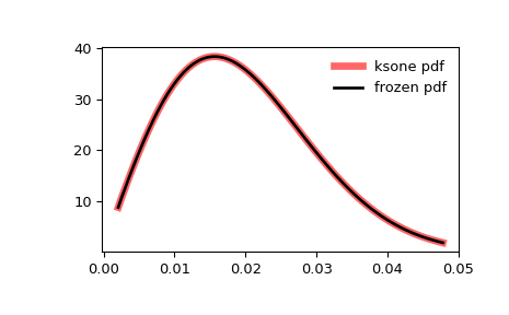
Display the probability density function (
pdf):>>> n = 1e+03 >>> x = np.linspace(ksone.ppf(0.01, n), ... ksone.ppf(0.99, n), 100) >>> ax.plot(x, ksone.pdf(x, n), ... 'r-', lw=5, alpha=0.6, label='ksone pdf')
Alternatively, the distribution object can be called (as a function) to fix the shape, location and scale parameters. This returns a “frozen” RV object holding the given parameters fixed.
Freeze the distribution and display the frozen
pdf:>>> rv = ksone(n) >>> ax.plot(x, rv.pdf(x), 'k-', lw=2, label='frozen pdf') >>> ax.legend(loc='best', frameon=False) >>> plt.show()
Check accuracy of
cdfandppf:>>> vals = ksone.ppf([0.001, 0.5, 0.999], n) >>> np.allclose([0.001, 0.5, 0.999], ksone.cdf(vals, n)) True