scipy.stats.genhyperbolic#
- scipy.stats.genhyperbolic = <scipy.stats._continuous_distns.genhyperbolic_gen object>[source]#
A generalized hyperbolic continuous random variable.
As an instance of the
rv_continuousclass,genhyperbolicobject inherits from it a collection of generic methods (see below for the full list), and completes them with details specific for this particular distribution.Methods
rvs(p, a, b, loc=0, scale=1, size=1, random_state=None)
Random variates.
pdf(x, p, a, b, loc=0, scale=1)
Probability density function.
logpdf(x, p, a, b, loc=0, scale=1)
Log of the probability density function.
cdf(x, p, a, b, loc=0, scale=1)
Cumulative distribution function.
logcdf(x, p, a, b, loc=0, scale=1)
Log of the cumulative distribution function.
sf(x, p, a, b, loc=0, scale=1)
Survival function (also defined as
1 - cdf, but sf is sometimes more accurate).logsf(x, p, a, b, loc=0, scale=1)
Log of the survival function.
ppf(q, p, a, b, loc=0, scale=1)
Percent point function (inverse of
cdf— percentiles).isf(q, p, a, b, loc=0, scale=1)
Inverse survival function (inverse of
sf).moment(order, p, a, b, loc=0, scale=1)
Non-central moment of the specified order.
stats(p, a, b, loc=0, scale=1, moments=’mv’)
Mean(‘m’), variance(‘v’), skew(‘s’), and/or kurtosis(‘k’).
entropy(p, a, b, loc=0, scale=1)
(Differential) entropy of the RV.
fit(data)
Parameter estimates for generic data. See scipy.stats.rv_continuous.fit for detailed documentation of the keyword arguments.
expect(func, args=(p, a, b), loc=0, scale=1, lb=None, ub=None, conditional=False, **kwds)
Expected value of a function (of one argument) with respect to the distribution.
median(p, a, b, loc=0, scale=1)
Median of the distribution.
mean(p, a, b, loc=0, scale=1)
Mean of the distribution.
var(p, a, b, loc=0, scale=1)
Variance of the distribution.
std(p, a, b, loc=0, scale=1)
Standard deviation of the distribution.
interval(confidence, p, a, b, loc=0, scale=1)
Confidence interval with equal areas around the median.
See also
Notes
The probability density function for
genhyperbolicis:\[f(x, p, a, b) = \frac{(a^2 - b^2)^{p/2}} {\sqrt{2\pi}a^{p-1/2} K_p\Big(\sqrt{a^2 - b^2}\Big)} e^{bx} \times \frac{K_{p - 1/2} (a \sqrt{1 + x^2})} {(\sqrt{1 + x^2})^{1/2 - p}}\]for \(x, p \in ( - \infty; \infty)\), \(|b| < a\) if \(p \ge 0\), \(|b| \le a\) if \(p < 0\). \(K_{p}(.)\) denotes the modified Bessel function of the second kind and order \(p\) (
scipy.special.kv)genhyperbolictakespas a tail parameter,aas a shape parameter,bas a skewness parameter.The probability density above is defined in the “standardized” form. To shift and/or scale the distribution use the
locandscaleparameters. Specifically,genhyperbolic.pdf(x, p, a, b, loc, scale)is identically equivalent togenhyperbolic.pdf(y, p, a, b) / scalewithy = (x - loc) / scale. Note that shifting the location of a distribution does not make it a “noncentral” distribution; noncentral generalizations of some distributions are available in separate classes.The original parameterization of the Generalized Hyperbolic Distribution is found in [1] as follows
\[f(x, \lambda, \alpha, \beta, \delta, \mu) = \frac{(\gamma/\delta)^\lambda}{\sqrt{2\pi}K_\lambda(\delta \gamma)} e^{\beta (x - \mu)} \times \frac{K_{\lambda - 1/2} (\alpha \sqrt{\delta^2 + (x - \mu)^2})} {(\sqrt{\delta^2 + (x - \mu)^2} / \alpha)^{1/2 - \lambda}}\]for \(x \in ( - \infty; \infty)\), \(\gamma := \sqrt{\alpha^2 - \beta^2}\), \(\lambda, \mu \in ( - \infty; \infty)\), \(\delta \ge 0, |\beta| < \alpha\) if \(\lambda \ge 0\), \(\delta > 0, |\beta| \le \alpha\) if \(\lambda < 0\).
The location-scale-based parameterization implemented in SciPy is based on [2], where \(a = \alpha\delta\), \(b = \beta\delta\), \(p = \lambda\), \(scale=\delta\) and \(loc=\mu\)
Moments are implemented based on [3] and [4].
For the distributions that are a special case such as Student’s t, it is not recommended to rely on the implementation of genhyperbolic. To avoid potential numerical problems and for performance reasons, the methods of the specific distributions should be used.
References
[1]O. Barndorff-Nielsen, “Hyperbolic Distributions and Distributions on Hyperbolae”, Scandinavian Journal of Statistics, Vol. 5(3), pp. 151-157, 1978. https://www.jstor.org/stable/4615705
[2]Eberlein E., Prause K. (2002) The Generalized Hyperbolic Model: Financial Derivatives and Risk Measures. In: Geman H., Madan D., Pliska S.R., Vorst T. (eds) Mathematical Finance - Bachelier Congress 2000. Springer Finance. Springer, Berlin, Heidelberg. DOI:10.1007/978-3-662-12429-1_12
[3]Scott, David J, Würtz, Diethelm, Dong, Christine and Tran, Thanh Tam, (2009), Moments of the generalized hyperbolic distribution, MPRA Paper, University Library of Munich, Germany, https://EconPapers.repec.org/RePEc:pra:mprapa:19081.
[4]E. Eberlein and E. A. von Hammerstein. Generalized hyperbolic and inverse Gaussian distributions: Limiting cases and approximation of processes. FDM Preprint 80, April 2003. University of Freiburg. https://freidok.uni-freiburg.de/fedora/objects/freidok:7974/datastreams/FILE1/content
Examples
>>> import numpy as np
>>> from scipy.stats import genhyperbolic
>>> import matplotlib.pyplot as plt
>>> fig, ax = plt.subplots(1, 1)
Get the support:
>>> p, a, b = 0.5, 1.5, -0.5
>>> lb, ub = genhyperbolic.support(p, a, b)
Calculate the first four moments:
>>> mean, var, skew, kurt = genhyperbolic.stats(p, a, b, moments='mvsk')
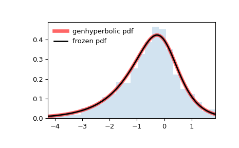
Display the probability density function (
pdf):>>> x = np.linspace(genhyperbolic.ppf(0.01, p, a, b), ... genhyperbolic.ppf(0.99, p, a, b), 100) >>> ax.plot(x, genhyperbolic.pdf(x, p, a, b), ... 'r-', lw=5, alpha=0.6, label='genhyperbolic pdf')
Alternatively, the distribution object can be called (as a function) to fix the shape, location and scale parameters. This returns a “frozen” RV object holding the given parameters fixed.
Freeze the distribution and display the frozen
pdf:>>> rv = genhyperbolic(p, a, b) >>> ax.plot(x, rv.pdf(x), 'k-', lw=2, label='frozen pdf')
Check accuracy of
cdfandppf:>>> vals = genhyperbolic.ppf([0.001, 0.5, 0.999], p, a, b) >>> np.allclose([0.001, 0.5, 0.999], genhyperbolic.cdf(vals, p, a, b)) True
Generate random numbers:
>>> r = genhyperbolic.rvs(p, a, b, size=1000)
And compare the histogram:
>>> ax.hist(r, density=True, bins='auto', histtype='stepfilled', alpha=0.2)
>>> ax.set_xlim([x[0], x[-1]])
>>> ax.legend(loc='best', frameon=False)
>>> plt.show()
