scipy.stats.

estimated_cdf#

scipy.stats.estimated_cdf(x, y, *, method='linear', axis=0, nan_policy='propagate', keepdims=None)[source]#

Estimate the CDF of the distribution underlying a sample.

Parameters:

xarray_like of real numbers

Data array.

yarray_like of real numbers

Points at which to evaluate the estimated cdf. See axis, keepdims, and the examples for broadcasting behavior.

methodstr, default: ‘linear’

The method to use for estimating the cumulative distribution function. The available options, numbered as they appear in [1], are:

‘inverted_cdf’ (AKA the empirical cumulative distribution function)
‘averaged_inverted_cdf’
‘closest_observation’
‘interpolated_inverted_cdf’
‘hazen’
‘weibull’
‘linear’ (default)
‘median_unbiased’
‘normal_unbiased’

See Notes for details.

axisint or None, default: 0

Axis along which samples in x are given in ND case. None ravels both x and y before performing the calculation, without checking whether the original shapes were compatible. As in other scipy.stats functions, a positive integer axis is resolved after prepending 1s to the shape of x or y as needed until the two arrays have the same dimensionality. When providing x and y with different dimensionality, consider using negative axis integers for clarity.

nan_policystr, default: ‘propagate’

Defines how to handle NaNs in the input data x.

propagate: if a NaN is present in the axis slice (e.g. row) along which the statistic is computed, the corresponding slice of the output will contain NaN(s).
omit: NaNs will be omitted when performing the calculation. If insufficient data remains in the axis slice along which the statistic is computed, the corresponding slice of the output will contain NaN(s).
raise: if a NaN is present, a ValueError will be raised.

If NaNs are present in y, the corresponding entries in the output will be NaN.

keepdimsbool, optional

Consider the case in which x is 1-D and y is a scalar: the estimated cumulative distribution function at a point is a reducing statistic, and the default behavior is to return a scalar. If keepdims is set to True, the axis will not be reduced away, and the result will be a 1-D array with one element.

The general case is more subtle, since multiple values of y may be specified for each axis-slice of x. For instance, if both x and y are 1-D and y.size > 1, no axis can be reduced away; there must be an axis to contain the number of values given by y.size. Therefore:

By default, the axis will be reduced away if possible (i.e. if there is exactly one element of y per axis-slice of x).
If keepdims is set to True, the axis will not be reduced away.
If keepdims is set to False, the axis will be reduced away if possible, and an error will be raised otherwise.

Returns:

probabilityscalar or ndarray: The resulting probabilities(s). The dtype is the result dtype of x, y, and the Python float type.

See also

quantile

Notes

Given a sample x from an underlying distribution, estimated_cdf provides a nonparametric estimate of the cumulative distribution function.

By default, this is done by computing the “fractional index” p at which y would appear within z, a sorted copy of x:

p = 1 / (n - 1) * (j +  (     y - z[j])
                      / (z[j+1] - z[j]))

where the index j is that of the largest element of z that does not exceed y, and n is the number of elements in the sample. Note that if y is an element of z, then j is the index such that y = z[j], and the formula simplifies to the intuitive j / (n - 1). The full formula linearly interpolates between j / (n - 1) and (j + 1) / (n - 1).

This is a special case of the more general:

p = (j + (y - z[j]) / (z[j+1] - z[j] + 1 - m) / n

where m may be defined according to several different conventions. The preferred convention may be selected using the method parameter:

`method`	number in H&F	`m`
`interpolated_inverted_cdf`	4	`0`
`hazen`	5	`1/2`
`weibull`	6	`p`
`linear` (default)	7	`1 - p`
`median_unbiased`	8	`p/3 + 1/3`
`normal_unbiased`	9	`p/4 + 3/8`

Note that indices j and j + 1 are clipped to the range 0 to n - 1 when the results of the formula would be outside the allowed range of non-negative indices, and resulting p is clipped to the range 0 to 1.

The table above includes only the estimators from [1] that are continuous functions of probability p (estimators 4-9). SciPy also provides the three discontinuous estimators from [1] (estimators 1-3), where j is defined as above, m is defined as follows, and g is 0 when index = p*n + m - 1 is less than 0 and otherwise is defined below.

inverted_cdf: m = 0 and g = int(index - j > 0)
averaged_inverted_cdf: m = 0 and g = (1 + int(index - j > 0)) / 2
closest_observation: m = -1/2 and g = 1 - int((index == j) & (j%2 == 1))

When all the data in x are unique, estimated_cdf and quantile are are inverses of one another within a certain domain. Although quantile with method='linear' is invertible over the whole domain of p from 0 to 1, this is not true of other methods.

Array API Standard Support

estimated_cdf has experimental support for Python Array API Standard compatible backends in addition to NumPy. Please consider testing these features by setting an environment variable SCIPY_ARRAY_API=1 and providing CuPy, PyTorch, JAX, or Dask arrays as array arguments. The following combinations of backend and device (or other capability) are supported.

Library	CPU	GPU
NumPy	✅	n/a
CuPy	n/a	✅
PyTorch	✅	✅
JAX	✅	✅
Dask	⛔	n/a

estimated_cdf also accepts MArrays backed by the backends indicated above; masked values will be treated as though they were not present.

See Support for the array API standard for more information.

References

[1] (1,2,3)

R. J. Hyndman and Y. Fan, “Sample quantiles in statistical packages,” The American Statistician, 50(4), pp. 361-365, 1996

Examples

>>> import numpy as np
>>> from scipy import stats
>>> x = [0, 1, 2, 3, 4, 5, 6, 7, 8, 9, 10]

Estimate the cumulative distribution function of one sample at a single point.

>>> stats.estimated_cdf(x, 5, axis=-1)
np.float64(0.5)

Estimate the cumulative distribution function of one sample at two points.

>>> stats.estimated_cdf(x, [2.5, 7.5], axis=-1)
array([0.25, 0.75])

Estimate the cumulative distribution function of two samples at different points.

>>> x = np.stack((np.arange(0, 11), np.arange(10, 21)))
>>> stats.estimated_cdf(x, [[2.5], [17.5]], axis=-1, keepdims=True)
array([[0.25],
       [0.75]])

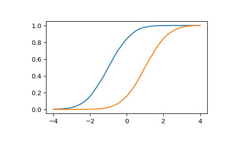
Estimate the cumulative distribution function at many points for each of two samples.

>>> import matplotlib.pyplot as plt
>>> rng = np.random.default_rng()
>>> x = stats.Normal(mu=[-1, 1]).sample(10000)
>>> y = np.linspace(-4, 4, 5000)[:, np.newaxis]
>>> p = stats.estimated_cdf(x, y, axis=0)
>>> plt.plot(y, p)
>>> plt.show()

../../_images/scipy-stats-estimated_cdf-1_00_00.png

Note that the quantile and estimated_cdf functions are inverses of one another within a certain domain.

>>> p = np.linspace(0, 1, 300)
>>> x = rng.standard_normal(300)
>>> y = stats.quantile(x, p)
>>> p2 = stats.estimated_cdf(x, y)
>>> np.testing.assert_allclose(p2, p)
>>> y2 = stats.quantile(x, p2)
>>> np.testing.assert_allclose(y2, y)

However, the domain over which quantile can be inverted by estimated_cdf depends on the method used. This is most noticeable when there are few observations in the sample.

>>> x = np.asarray([0, 1])
>>> y_linear = stats.quantile(x, p, method='linear')
>>> y_weibull = stats.quantile(x, p, method='weibull')
>>> y_iicdf = stats.quantile(x, p, method='interpolated_inverted_cdf')
>>> plt.plot(p, y_linear, p, y_weibull, p, y_iicdf)
>>> plt.legend(['linear', 'weibull', 'iicdf'])
>>> plt.xlabel('p')
>>> plt.ylabel('y = quantile(x, p)')
>>> plt.show()

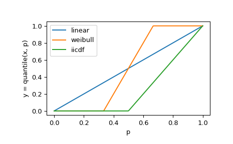
../../_images/scipy-stats-estimated_cdf-1_01_00.png

For example, in the case above, quantile is only invertible from p = 0.5 to p = 1.0 with method = 'interpolated_inverted_cdf'. This is a fundamental characteristic of the methods, not a shortcoming of estimated_cdf.