scipy.special.yv#
- scipy.special.yv(v, z, out=None) = <ufunc 'yv'>#
Bessel function of the second kind of real order and complex argument.
- Parameters:
- varray_like
Order (float).
- zarray_like
Argument (float or complex).
- outndarray, optional
Optional output array for the function results
- Returns:
- Yscalar or ndarray
Value of the Bessel function of the second kind, \(Y_v(x)\).
See also
Notes
For positive v values, the computation is carried out using the AMOS [1] zbesy routine, which exploits the connection to the Hankel Bessel functions \(H_v^{(1)}\) and \(H_v^{(2)}\),
\[Y_v(z) = \frac{1}{2\imath} (H_v^{(1)} - H_v^{(2)}).\]For negative v values the formula,
\[Y_{-v}(z) = Y_v(z) \cos(\pi v) + J_v(z) \sin(\pi v)\]is used, where \(J_v(z)\) is the Bessel function of the first kind, computed using the AMOS routine zbesj. Note that the second term is exactly zero for integer v; to improve accuracy the second term is explicitly omitted for v values such that v = floor(v).
References
[1]Donald E. Amos, “AMOS, A Portable Package for Bessel Functions of a Complex Argument and Nonnegative Order”, http://netlib.org/amos/
Examples
Evaluate the function of order 0 at one point.
>>> from scipy.special import yv
>>> yv(0, 1.)
0.088256964215677
Evaluate the function at one point for different orders.
>>> yv(0, 1.), yv(1, 1.), yv(1.5, 1.)
(0.088256964215677, -0.7812128213002889, -1.102495575160179)
The evaluation for different orders can be carried out in one call by providing a list or NumPy array as argument for the v parameter:
>>> yv([0, 1, 1.5], 1.)
array([ 0.08825696, -0.78121282, -1.10249558])
Evaluate the function at several points for order 0 by providing an array for z.
>>> import numpy as np
>>> points = np.array([0.5, 3., 8.])
>>> yv(0, points)
array([-0.44451873,  0.37685001,  0.22352149])
If z is an array, the order parameter v must be broadcastable to the correct shape if different orders shall be computed in one call. To calculate the orders 0 and 1 for a 1D array:
>>> orders = np.array([[0], [1]])
>>> orders.shape
(2, 1)
>>> yv(orders, points)
array([[-0.44451873,  0.37685001,  0.22352149],
       [-1.47147239,  0.32467442, -0.15806046]])
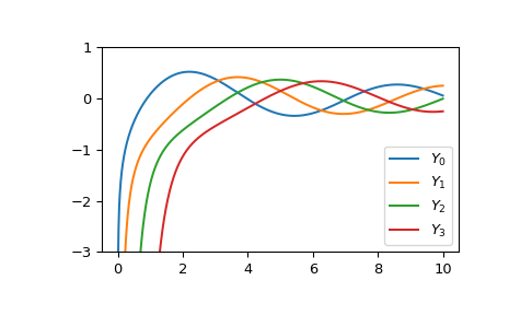
Plot the functions of order 0 to 3 from 0 to 10.
>>> import matplotlib.pyplot as plt
>>> fig, ax = plt.subplots()
>>> x = np.linspace(0., 10., 1000)
>>> for i in range(4):
...     ax.plot(x, yv(i, x), label=f'$Y_{i!r}$')
>>> ax.set_ylim(-3, 1)
>>> ax.legend()
>>> plt.show()