scipy.special.tklmbda#

scipy.special.tklmbda(x, lmbda, out=None) = <ufunc 'tklmbda'>#

Cumulative distribution function of the Tukey lambda distribution.

Parameters:

x, lmbdaarray_like: Parameters
outndarray, optional: Optional output array for the function results

Returns:

cdfscalar or ndarray: Value of the Tukey lambda CDF

See also

scipy.stats.tukeylambda: Tukey lambda distribution

Examples

>>> import numpy as np
>>> import matplotlib.pyplot as plt
>>> from scipy.special import tklmbda, expit

Compute the cumulative distribution function (CDF) of the Tukey lambda distribution at several x values for lmbda = -1.5.

>>> x = np.linspace(-2, 2, 9)
>>> x
array([-2. , -1.5, -1. , -0.5,  0. ,  0.5,  1. ,  1.5,  2. ])
>>> tklmbda(x, -1.5)
array([0.34688734, 0.3786554 , 0.41528805, 0.45629737, 0.5       ,
       0.54370263, 0.58471195, 0.6213446 , 0.65311266])

When lmbda is 0, the function is the logistic sigmoid function, which is implemented in scipy.special as expit.

>>> tklmbda(x, 0)
array([0.11920292, 0.18242552, 0.26894142, 0.37754067, 0.5       ,
       0.62245933, 0.73105858, 0.81757448, 0.88079708])
>>> expit(x)
array([0.11920292, 0.18242552, 0.26894142, 0.37754067, 0.5       ,
       0.62245933, 0.73105858, 0.81757448, 0.88079708])

When lmbda is 1, the Tukey lambda distribution is uniform on the interval [-1, 1], so the CDF increases linearly.

>>> t = np.linspace(-1, 1, 9)
>>> tklmbda(t, 1)
array([0.   , 0.125, 0.25 , 0.375, 0.5  , 0.625, 0.75 , 0.875, 1.   ])

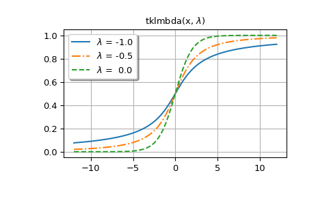
In the following, we generate plots for several values of lmbda.

The first figure shows graphs for lmbda <= 0.

>>> styles = ['-', '-.', '--', ':']
>>> fig, ax = plt.subplots()
>>> x = np.linspace(-12, 12, 500)
>>> for k, lmbda in enumerate([-1.0, -0.5, 0.0]):
...     y = tklmbda(x, lmbda)
...     ax.plot(x, y, styles[k], label=rf'$\lambda$ = {lmbda:-4.1f}')

>>> ax.set_title(r'tklmbda(x, $\lambda$)')
>>> ax.set_label('x')
>>> ax.legend(framealpha=1, shadow=True)
>>> ax.grid(True)

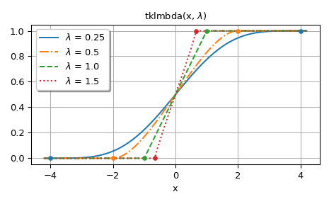
The second figure shows graphs for lmbda > 0. The dots in the graphs show the bounds of the support of the distribution.

>>> fig, ax = plt.subplots()
>>> x = np.linspace(-4.2, 4.2, 500)
>>> lmbdas = [0.25, 0.5, 1.0, 1.5]
>>> for k, lmbda in enumerate(lmbdas):
...     y = tklmbda(x, lmbda)
...     ax.plot(x, y, styles[k], label=fr'$\lambda$ = {lmbda}')

>>> ax.set_prop_cycle(None)
>>> for lmbda in lmbdas:
...     ax.plot([-1/lmbda, 1/lmbda], [0, 1], '.', ms=8)

>>> ax.set_title(r'tklmbda(x, $\lambda$)')
>>> ax.set_xlabel('x')
>>> ax.legend(framealpha=1, shadow=True)
>>> ax.grid(True)

>>> plt.tight_layout()
>>> plt.show()

../../_images/scipy-special-tklmbda-1_00_00.png

../../_images/scipy-special-tklmbda-1_00_01.png

The CDF of the Tukey lambda distribution is also implemented as the cdf method of scipy.stats.tukeylambda. In the following, tukeylambda.cdf(x, -0.5) and tklmbda(x, -0.5) compute the same values:

>>> from scipy.stats import tukeylambda
>>> x = np.linspace(-2, 2, 9)

>>> tukeylambda.cdf(x, -0.5)
array([0.21995157, 0.27093858, 0.33541677, 0.41328161, 0.5       ,
       0.58671839, 0.66458323, 0.72906142, 0.78004843])

>>> tklmbda(x, -0.5)
array([0.21995157, 0.27093858, 0.33541677, 0.41328161, 0.5       ,
       0.58671839, 0.66458323, 0.72906142, 0.78004843])

The implementation in tukeylambda also provides location and scale parameters, and other methods such as pdf() (the probability density function) and ppf() (the inverse of the CDF), so for working with the Tukey lambda distribution, tukeylambda is more generally useful. The primary advantage of tklmbda is that it is significantly faster than tukeylambda.cdf.