scipy.special.sici#

scipy.special.sici(x, out=None) = <ufunc 'sici'>#

Sine and cosine integrals.

The sine integral is

\[\int_0^x \frac{\sin{t}}{t}dt\]

and the cosine integral is

\[\gamma + \log(x) + \int_0^x \frac{\cos{t} - 1}{t}dt\]

where \(\gamma\) is Euler’s constant and \(\log\) is the principal branch of the logarithm [1].

Parameters:

xarray_like: Real or complex points at which to compute the sine and cosine integrals.
outtuple of ndarray, optional: Optional output arrays for the function results

Returns:

siscalar or ndarray: Sine integral at x
ciscalar or ndarray: Cosine integral at x

See also

shichi: Hyperbolic sine and cosine integrals.
exp1: Exponential integral E1.
expi: Exponential integral Ei.

Notes

For real arguments with x < 0, ci is the real part of the cosine integral. For such points ci(x) and ci(x + 0j) differ by a factor of 1j*pi.

For real arguments the function is computed by calling Cephes’ [2] sici routine. For complex arguments the algorithm is based on Mpmath’s [3] si and ci routines.

References

[1] (1,2)

Milton Abramowitz and Irene A. Stegun, eds. Handbook of Mathematical Functions with Formulas, Graphs, and Mathematical Tables. New York: Dover, 1972. (See Section 5.2.)

[2]

Cephes Mathematical Functions Library, http://www.netlib.org/cephes/

[3]

Fredrik Johansson and others. “mpmath: a Python library for arbitrary-precision floating-point arithmetic” (Version 0.19) http://mpmath.org/

Examples

>>> import numpy as np
>>> import matplotlib.pyplot as plt
>>> from scipy.special import sici, exp1

sici accepts real or complex input:

>>> sici(2.5)
(1.7785201734438267, 0.2858711963653835)
>>> sici(2.5 + 3j)
((4.505735874563953+0.06863305018999577j),
(0.0793644206906966-2.935510262937543j))

For z in the right half plane, the sine and cosine integrals are related to the exponential integral E1 (implemented in SciPy as scipy.special.exp1) by

Si(z) = (E1(i*z) - E1(-i*z))/2i + pi/2
Ci(z) = -(E1(i*z) + E1(-i*z))/2

See [1] (equations 5.2.21 and 5.2.23).

We can verify these relations:

>>> z = 2 - 3j
>>> sici(z)
((4.54751388956229-1.3991965806460565j),
(1.408292501520851+2.9836177420296055j))

>>> (exp1(1j*z) - exp1(-1j*z))/2j + np.pi/2  # Same as sine integral
(4.54751388956229-1.3991965806460565j)

>>> -(exp1(1j*z) + exp1(-1j*z))/2            # Same as cosine integral
(1.408292501520851+2.9836177420296055j)

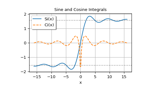
Plot the functions evaluated on the real axis; the dotted horizontal lines are at pi/2 and -pi/2:

>>> x = np.linspace(-16, 16, 150)
>>> si, ci = sici(x)

>>> fig, ax = plt.subplots()
>>> ax.plot(x, si, label='Si(x)')
>>> ax.plot(x, ci, '--', label='Ci(x)')
>>> ax.legend(shadow=True, framealpha=1, loc='upper left')
>>> ax.set_xlabel('x')
>>> ax.set_title('Sine and Cosine Integrals')
>>> ax.axhline(np.pi/2, linestyle=':', alpha=0.5, color='k')
>>> ax.axhline(-np.pi/2, linestyle=':', alpha=0.5, color='k')
>>> ax.grid(True)
>>> plt.show()