scipy.special.

jacobi#

scipy.special.jacobi(n, alpha, beta, monic=False)[source]#

Jacobi polynomial.

Defined to be the solution of

(1 - x^{2}) \frac{d^{2}}{d x^{2}} P_{n}^{(α, β)} + (β - α - (α + β + 2) x) \frac{d}{d x} P_{n}^{(α, β)} + n (n + α + β + 1) P_{n}^{(α, β)} = 0

$(1 - x^2)\frac{d^2}{dx^2}P_n^{(\alpha, \beta)} + (\beta - \alpha - (\alpha + \beta + 2)x) \frac{d}{dx}P_n^{(\alpha, \beta)} + n(n + \alpha + \beta + 1)P_n^{(\alpha, \beta)} = 0$

for $\alpha, \beta > -1$ ; $P_n^{(\alpha, \beta)}$ is a polynomial of degree $n$ .

Parameters:

nint: Degree of the polynomial.
alphafloat: Parameter, must be greater than -1.
betafloat: Parameter, must be greater than -1.
monicbool, optional: If True, scale the leading coefficient to be 1. Default is False.

Returns:

Porthopoly1d: Jacobi polynomial.

Notes

For fixed $\alpha, \beta$ , the polynomials $P_n^{(\alpha, \beta)}$ are orthogonal over $[-1, 1]$ with weight function $(1 - x)^\alpha(1 + x)^\beta$ .

References

[AS]

Milton Abramowitz and Irene A. Stegun, eds. Handbook of Mathematical Functions with Formulas, Graphs, and Mathematical Tables. New York: Dover, 1972.

Examples

The Jacobi polynomials satisfy the recurrence relation:

P_{n}^{(α, β - 1)} (x) - P_{n}^{(α - 1, β)} (x) = P_{n - 1}^{(α, β)} (x)

$P_n^{(\alpha, \beta-1)}(x) - P_n^{(\alpha-1, \beta)}(x) = P_{n-1}^{(\alpha, \beta)}(x)$

This can be verified, for example, for $\alpha = \beta = 2$ and $n = 1$ over the interval $[-1, 1]$ :

>>> import numpy as np
>>> from scipy.special import jacobi
>>> x = np.arange(-1.0, 1.0, 0.01)
>>> np.allclose(jacobi(0, 2, 2)(x),
...             jacobi(1, 2, 1)(x) - jacobi(1, 1, 2)(x))
True

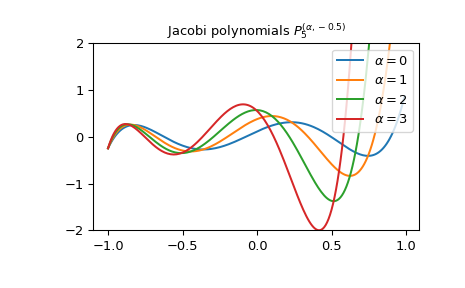
Plot of the Jacobi polynomial $P_5^{(\alpha, -0.5)}$ for different values of $\alpha$ :

>>> import matplotlib.pyplot as plt
>>> x = np.arange(-1.0, 1.0, 0.01)
>>> fig, ax = plt.subplots()
>>> ax.set_ylim(-2.0, 2.0)
>>> ax.set_title(r'Jacobi polynomials $P_5^{(\alpha, -0.5)}$')
>>> for alpha in np.arange(0, 4, 1):
...     ax.plot(x, jacobi(5, alpha, -0.5)(x), label=rf'$\alpha={alpha}$')
>>> plt.legend(loc='best')
>>> plt.show()

../../_images/scipy-special-jacobi-1.png