scipy.special.

gegenbauer#

scipy.special.gegenbauer(n, alpha, monic=False)[source]#

Gegenbauer (ultraspherical) polynomial.

Defined to be the solution of

\[(1 - x^2)\frac{d^2}{dx^2}C_n^{(\alpha)} - (2\alpha + 1)x\frac{d}{dx}C_n^{(\alpha)} + n(n + 2\alpha)C_n^{(\alpha)} = 0\]

for \(\alpha > -1/2\); \(C_n^{(\alpha)}\) is a polynomial of degree \(n\).

Parameters:

nint: Degree of the polynomial.
alphafloat: Parameter, must be greater than -0.5.
monicbool, optional: If True, scale the leading coefficient to be 1. Default is False.

Returns:

Corthopoly1d: Gegenbauer polynomial.

Notes

The polynomials \(C_n^{(\alpha)}\) are orthogonal over \([-1,1]\) with weight function \((1 - x^2)^{(\alpha - 1/2)}\).

Examples

>>> import numpy as np
>>> from scipy import special
>>> import matplotlib.pyplot as plt

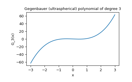
We can initialize a variable p as a Gegenbauer polynomial using the gegenbauer function and evaluate at a point x = 1.

>>> p = special.gegenbauer(3, 0.5, monic=False)
>>> p
poly1d([ 2.5,  0. , -1.5,  0. ])
>>> p(1)
1.0

To evaluate p at various points x in the interval (-3, 3), simply pass an array x to p as follows:

>>> x = np.linspace(-3, 3, 400)
>>> y = p(x)

We can then visualize x, y using matplotlib.pyplot.

>>> fig, ax = plt.subplots()
>>> ax.plot(x, y)
>>> ax.set_title("Gegenbauer (ultraspherical) polynomial of degree 3")
>>> ax.set_xlabel("x")
>>> ax.set_ylabel("G_3(x)")
>>> plt.show()

../../_images/scipy-special-gegenbauer-1.png